Let us start with the two most burning questions: What is geo-spatial data and what is a GIS?
Geo-spatial data in the simplest terms is any type of data referenced to a specific location on Earth. It consists broadly of two elements: 1) location data (where things are) and 2) attributes data (what things are like there). Location data allows us to position our data values adequately on the surface of the Earth. Attributes data describes any features of that specific location (temperature, elevation, road type, a bridge, demographic information and so on).
Geographic Information System (GIS) is a system that creates, manages, analyses, and maps data. GIS connects data to a map, integrating location data with all types of descriptive information.
4.1 Geo-spatial data sources
4.1.1 Traditional surveys
Recall that geo-spatial data is simply a set of data values that are indexed to a geographical location on Earth. In that sense, traditional census or surveys are sources of geo-spatial data as long as they contain information on administrative units, GPS location, or any other geographical identifiers. Data coming from traditional surveys can even be more precise, for instance if we are interested in measuring a building and its properties.
4.1.2 Remote sensing
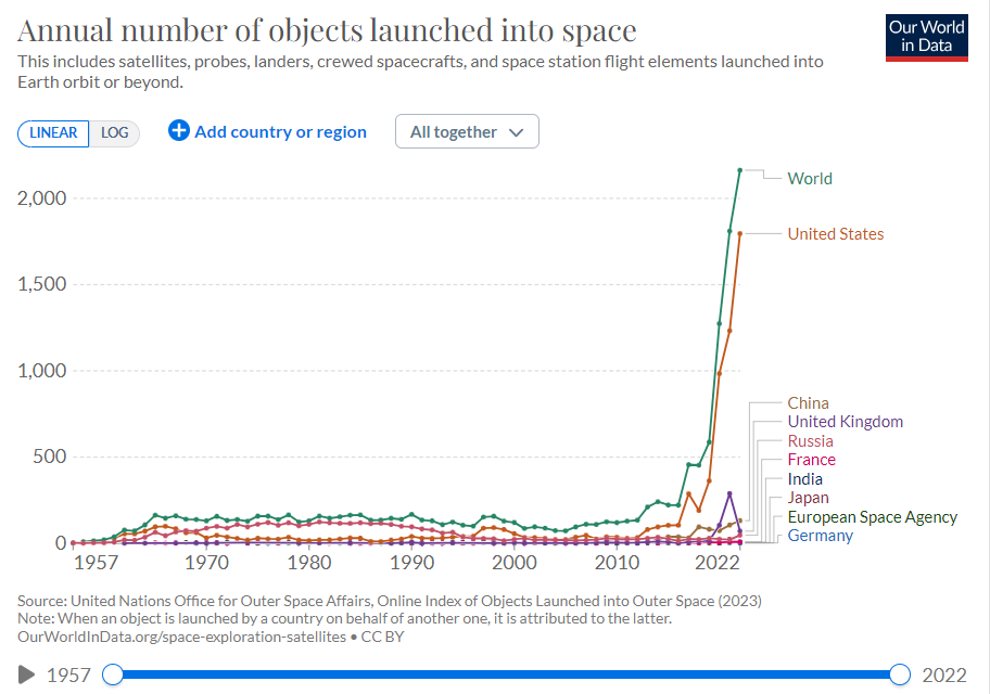
Increasingly, remote sensing data collection is turning out to be a very efficient way of collection geo-spatial data. This includes satellite imagery and aircraft sensors that orbit the Earth and collect data continuously, at a high spatial resolution, and globally, including places that would be hard to reach with a survey (say the middle of the ocean or conflict-affected areas). In fact, due to the advantages of remote sensing data collection - space is becoming a crowded place, and increasingly more so in the last couple of years. Figure 4.1 below shows the time trend of the annual number of objects launched into space, which explodes upwards after around 2015. As of 2022, there were 6,905 active satellites in space. In this workflow, we will be relying heavily on remote sensing data, but let us briefly consider other sources of geo-spatial information.
For all the growing interest in remote sensing data collection, it is worth acknowledging that highly valuable geo-spatial information often comes from humans on the ground! Crowdsourcing geo-spatial data is often done via informal social networks and does not require any formal training in geo-spatial technologies. Perhaps one of the most notable examples is Open Street Map (OSM), a community of mappers with local knowledge that produce open source maps. The Humanitarian team at OSM produces community-developed maps in areas such as Disasters & Climate Resilience or Public Health - for example, OSM is working with the World Bank and the Caribbean Disaster Emergency Management Agency (CDEMA) to integrate their maps into official disaster risk response.
4.1.4 Cell phone data
Basic services provided by cell phone operators are routed by satellites, providing location information at various levels of precision (from GPS to cell phone tower), together with Call Detail Records (CDR). Flowminder is an example of an organisation that leverages mobile operator data in development projects, for instance tracking population movements post the 2015 Nepal Earthquake.
4.1.5 Online data
Online data is broad and includes all data shared online purposefully, including Wikipedia, social media, online articles etc. Location and mobility tracking via social media can be another source of geographical information. App-based mobile phone location data is actually often of higher spatial resolution than that coming from cell phone data operators and is increasingly being used in mobility studies.
4.2 Data structures
We want to introduce the two most common spatial data types, which we will be working with in our poverty mapping exercise, together with their attributes.
Important
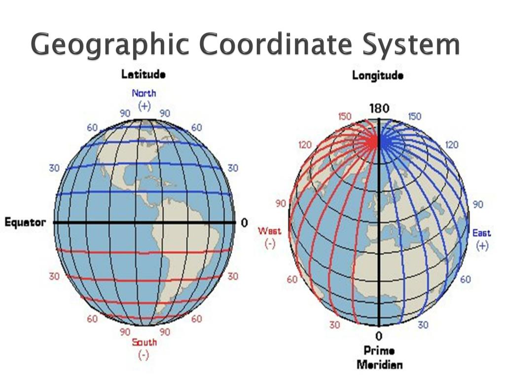
An important note on the naming conventions and structures of geographical coordinates in geo-spatial data. A set of coordinates will typically be expressed as (x,y), where x relates to longitude and y to latitude. Latitude has a range (-90, 90), while longitude has a range (-180, 180). Negative values of longitude refer to the Western hemisphere and positive values to the Eastern hemisphere. Similarly, negative values of latitude refer to the Southern hemisphere and positive values refer to the Northern hemisphere. See Figure 4.2 for a diagram that can serve as a cheat sheet!
Figure 4.2: Geographic Coordinate System
4.2.1 Raster data
Raster data is a collection of cells (or pixels) organised into rows and columns (called a grid), defined by its location in space. The raster is the pattern of locations that together - as a grid - cover a geographic area. Cells have values that carry information about those locations, such as temperature or elevation. Values can be continuous (e.g. a range of temperature values), or categorical (e.g. different categories of land use). If pixels sound familiar, it’s because they are - in fact, this is how every digital image is represented. The only difference is that a raster additionally includes spatial information that connects data from the image to a particular location. The location is defined by the following attributes (these are important attributes to inspect when you first open your raster):
Extent
Cell size (spatial resolution or size of each pixel)
The number of rows and columns
Coordinate Reference System (CRS)
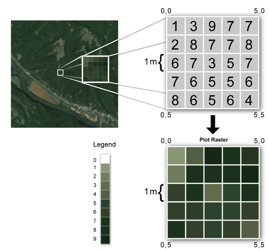
To illustrate this concept, below is Figure 4.3 with a raster image showing the elevation of Harvard Forest. Each pixel has values of elevation assigned, which range from 0-9. Here, the spatial resolution is 1m x 1m, which means each pixel has an area of 1m by 1m (this is really granular!).
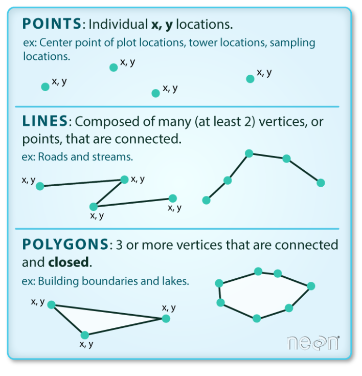
Vector data represents structures on the Earth’s surface that are defined by discrete locations (x,y) called vertices. Depending on how the vertices (x,y) are oragnised, we can divide vector data types into: points, lines, and polygons. You could think of: locations of hospitals, road networks, administrative boundaries. See Figure 4.4 for a representation of different geometries.
We could add another category to this, which is the multipolygon. As the name suggests, a multipolygon is a collection of polygons. For instance, if we think about a polygon representing a lake or a forest cover, a multipolygon could depict an area of a national park that consists of a forest cover and two lakes - such as in the image below. In this particular example our polygons are nested within each other, but they could very well be just next to each other and not touching (such as two buildings on either side of a street).
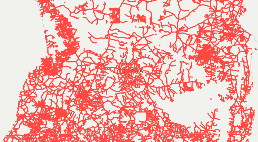
To illustrate the concept further, Figure 4.5 shows a vector data set with lines showing the road network in Ghana, developed through Open Street Maps Ghana, downloadable via the Humanitarian Data Exchange website. Each line is determined by its vertices (think of them as the (x,y) points shown in the image above) and indexed geographically in space.
Vector data comes in many formats, but we will be working with the (very common) Shapefile format, which has a .shp extension. More specifically, we will download a shapefile containing multipolygons that define administrative boundaries of upazilas (admin level 3) in Bangladesh. A shapefile stores the coordinates of vertices, as well as other metadata:
Extent
Object type - whether the shapefile contains points, lines, or polygons.
Coordinate Reference System (CRS)
Other attributes - e.g. in our case the name of the upazila, its administrative code, area covered etc.
Quick quiz alert
Now, let’s do a super quick quiz to check our intuitition, which goes as follows: we will present to you a few examples of geo-spatial datasets and invite you to either type in the chat or shout out directly whether this is a vector or a raster dataset.
4.3 Layering geo-spatial data sets
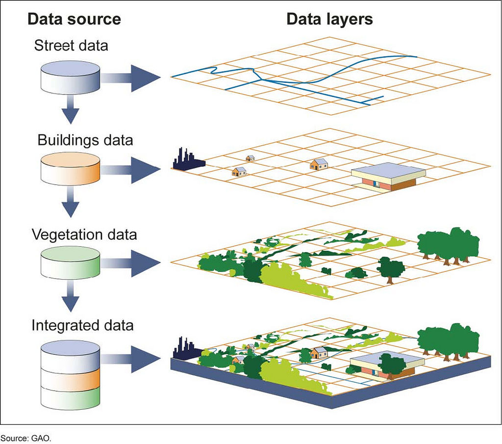
Now that you are familiar with the basic types of geo-spatial datasets, we can start thinking about performing some simple mapping. Typically, rather than viewing each layer of data (such as your road network, elevation, temperature etc.) individually, it is valuable to overlay them on top of each other, so that we can view multiple geo-spatial layers at the same time. The diagram in Figure 4.6 below demonstrates this concept: while we can inspect data on streets, buildings, and vegetation individually, a much more interesting way to look at these layers is by viewing the simultaneously, as in the “Integrated data” portion of the diagram at the very bottom.
Make sure that the CRS is the same for all of your objects before layering. The most standard CRS is the World Geodetic System 1984 (WGS 84), but you may encounter other ones when working with spatial data for specific regions of the world.
Now, let’s see an example of visualising multiple raster layers from our project work under Data & Evidence to End Extreme Poverty (DEEP). In this case, we wanted to map the spatial distribution of climatic risks in Nigeria, looking at droughts and floods. Figure 4.7 below shows the worst drought (defined as Standardized Precipitation Evapotranspiration Index or SPEI below -1.5) and all flooded areas in the period 2010-2020 in Nigeria, on top of an Open Street Map background. Drought is captured by a continuous variable for a range of values of SPEI (large pixels from yellow to red), while flood is a categorical variable (i.e. flood or no flood), with flooded areas shown in blue. We can see that the extent of these layers differs, i.e. drought is only defined within Nigeria (including bordering grid cells), while flood data extends beyond the borders of Nigeria and considers an entire river system, which is not necessarily bound by national borders.
Figure 4.7: Rasters showing all floods and the worst droughts in Nigeria between 2010-2020
The two layers (drought and flood) also have different spatial resolutions. Here, drought data is of a lower spatial resolution, i.e. it comes up as big pixels of around 0.5 degrees (or ~30km x 30km), while flood data is extremely high resolution, with each pixel the size of ~250m x 250m, coming from the NASA MODIS satellite. Figure 4.8 below shows a zoom into two grid cells of drought data, which contain numerous grid cells with flood data. The higher the spatial resolution, the smaller your grid cells!
Figure 4.8: Zoom into pixels showing floods and droughts in Nigeria
4.4 Raster manipulation for poverty modelling
The previous section introduced the concept of working with multiple layers of geo-spatial information. In our example, the two layers, despite being displayed on top of each other, had very different attributes: spatial resolution, cell sizes, extent . However, there are cases, as in the poverty modelling exercise we are about to do, where we want to “harmonise” our raster objects, i.e. make sure all the attributes (CRS, extent, spatial resolution, cell size) are the same when rasters are overlaid on top of each other.
Let’s consider our problem at hand again: We want to compute poverty statistics at administrative level 3 (upazila) level in Bangladesh. We will do so by using statistical modelling and a number of remote sensed covariates as our predictors. For this, we need some basic statistics (mean, min, max, standard deviation, count etc.) that describe geo-spatial information for each upazila. For example, what is the mean Travel Time to Healthcare Facilities (in minutes) in the upazila of Abador? Or, what is the median nightlights intensity in that upazila? While R is smart enough to compute those statistics for us automatically, we need to provide it with a nicely harmonised set of rasters. We will use a “base layer”, which contains all the attributes we are interested in, and harmonise all other remote sensing covariates to our base layer. That is: we will match the CRS, extent, spatial resolution, cell size of all our data to the one of the base layer.
With that in mind, we will introduce a few ways in which we will manipulate spatial data. This is a useful skill to have as we will soon discover that raw open source data can be a little messy and you may need to implement some of these steps to make sense of your data before any meaningful analysis.
Cropping - changing the extent of our spatial objects, i.e. the maximum and minimum values of longitude and latitude that define the object, to that of the base layer.
Resampling - changing the spatial resolution so that it matches that of the base layer.
Recoding missing values - (only if appropriate) changing missing values to a specified value.
Caution
A note of caution on missing values in geo-spatial data. As with every data type, the treatment of missing values can be a source of philosophical discussions and should always be determined depending on the context and the specific problem at hand. The user should always ask themselves: can a missing value be interpreted as a zero or do we simply not have enough information to conclude? If it is a zero, missing values can be recoded accordingly. Be careful with this. If in doubt, always consult an expert.
Masking - cutting the exact “shape” of a raster layer. This is different from cropping, which would leave us with a chunky box that contains Bangladesh, but also some areas between the maximum and minimum values that fall outside of Bangladesh. We can use the mask function to examine only the country boundaries.
These concepts may seem a little abstract for now, so let us consider visually what each of these processes will entail. Let’s take the example of processing geo-spatial data on nightlights intensity for Bangladesh - a process we will be implementing in Step 5 of Section 3. Night lights intensity has been widely used in literature as a proxy for income and will be one of our predictors of poverty. Figure 4.9 shows a TIFF file with the aerial shot of nightlights intensity in South-East Asia as seen from space. We can see that urban areas and areas with higher density of economic activity appear more luminous. We will use the functions described above to manipulate this TIFF file and transform it into a raster layer for Bangladesh with codified values of radiance per pixel (this is a measure of nightlights intensity).
Figure 4.9: Aerial image showing nightlights in East Asia
Figure 4.10 below shows the processing of data on nightlights intensity. The left hand side is what you will see if you simply load the above TIFF file into your R environment, turn it into a raster, and plot - in other words, a massive block of dark blue over Asia. The original raster shows values of nightlights intensity for the entire South East Asia region at the original spatial resolution of around ~450m.
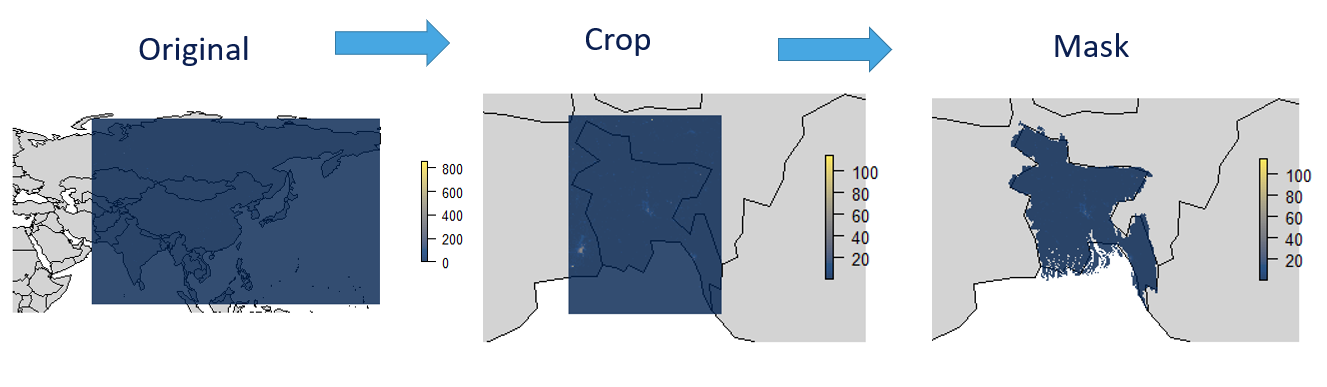
First, we are interested in analysing just Bangladesh, rather than the entirely of South East Asia (not least because TIFF files can be quite heavy and maintaining unnecessarily large raster objects slows down a lot of the computation). We will “crop” our raster object to the Bangladesh base layer, i.e. we will change the extent to that of Bangladesh. Now, our raster object changed dimensions. It is defined by the maximum and minimum values of longitude and latitude in Bangladesh.
We also want to view the “shape” of Bangladesh, rather than a rectangular box bound by its extent. For this purpose, we “mask” our raster layer with nightlights to the base layer - and we achieve a nicely formatted raster that resembles Bangladesh!
Just a note that along this process, we also resample the raster, i.e. change the spatial resolution to ~100m to match that of our base layer. Going from a lower to a higher spatial resolution is called disaggregation. If we zoomed into the image, we would see more of smaller pixels appear than previously. However, since the diagram is meant to demonstrate how we change the geographical coverage, it is quite zoomed out and luminous pixels in yellow do not appear immediately visible. Also, given that we are working with a really high spatial resolution - we would need to zoom a lot, possibly to the level of individual buildings, in order to see the change resulting from resampling (hence we do not show it in the diagram).
Figure 4.10: Processing of nightlights data
4.5 Spatial Data in R
Given that our entire workflow will be carried out in R to make it accessible, open source, and user-friendly - we will introduce some common spatial objects in R. There are numerous packages that allow you to work with spatial data. In fact, packages are very often retired and new ones are created to replace them. We will be relying mostly on:
Recently spatial data in R has been standardised using the base package sp. Although a newer version of this package exists, called sf , it is useful to understand basic data structures under sp. Let’s have a look at the spatial data classes by running the chunk below:
library(sp)
getClass("Spatial")
Class "Spatial" [package "sp"]

Slots:

Name:         bbox proj4string
Class:      matrix         CRS

Known Subclasses:
Class "SpatialPoints", directly
Class "SpatialMultiPoints", directly
Class "SpatialGrid", directly
Class "SpatialLines", directly
Class "SpatialPolygons", directly
Class "SpatialPointsDataFrame", by class "SpatialPoints", distance 2
Class "SpatialPixels", by class "SpatialPoints", distance 2
Class "SpatialMultiPointsDataFrame", by class "SpatialMultiPoints", distance 2
Class "SpatialGridDataFrame", by class "SpatialGrid", distance 2
Class "SpatialLinesDataFrame", by class "SpatialLines", distance 2
Class "SpatialPixelsDataFrame", by class "SpatialPoints", distance 3
Class "SpatialPolygonsDataFrame", by class "SpatialPolygons", distance 2
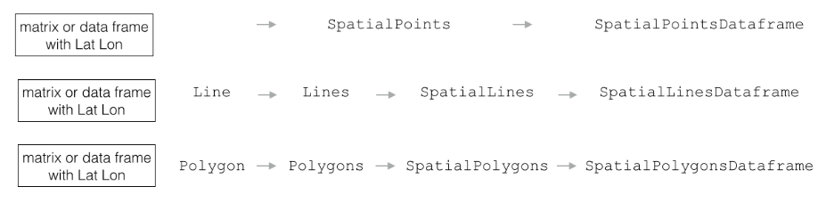
A basic sp object will have two “slots”: a bounding box bbox containing a matrix of longitude and latitude values (or, using the language we introduced earlier, the extent of an object) and proj4string, which is the CRS. These parameters will help us locate our object in space. The basis of all the spatial objects is a matrix or data frame with latitude and longitude values - this is what we need to make our existing objects in R “spatial”. From the output above, we can also see that objects build on each other. This is illustrated in Figure 4.11 below. For example, taking our matrix or data frame with latitude and longitude, we can create a SpatialPoints object, which would simply be a collection of spatial points. We can build on this and create a SpatialPointsDataFrame by adding a data frame with attributes associated with these points. The same can be done for lines and polygons.
Figure 4.11: Spatial objects in R
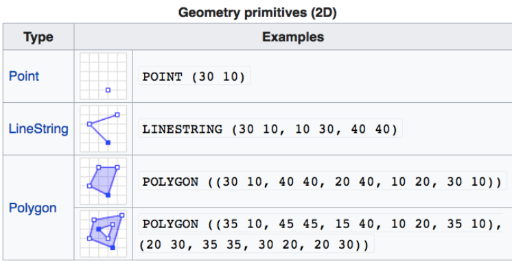
4.5.2 Vector data with sf package
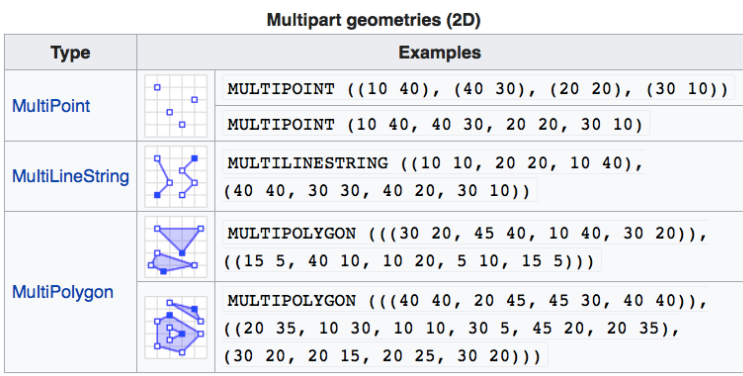
The sf package implements Simple Features, which is a set of standards that specify storage and model of geographic features used in geographic information systems. It is famous enough to have its Wikipedia page and is endorsed by the Open Geospatial Consortium. It works only with vector data and does not accommodate rasters. Common geometry types are shown in Figure 4.12 below. Among the primitive ones, we have Points, LineStrings, and Polygons (the same as simple vector geometry types discussed in Section 2.2.) The sf package allows for multipart geometries, essentially a collection of primitive geometries, such as: MultiPoints, MultiLineString, and MultiPolygons, shown in Figure 4.13 below. The coordinates in brackets specify each vertex that defines the geometry.
sf objects are organised into three elements. Figure 4.14 shows an example of an sf object, which displays 100 features (or rows in our data) and 6 fields (columns in our data). The key elements that make up this object are:
sf, an individual row or record in our data with values for each column (green box).
sfc, the simple feature geometry list-column (red box). This column indicates that our object is indeed ‘spatial’, as opposed to being a simple data frame. It contains the geometry type for each row in our data (see geometry types we learned in the figure above: they could be lines, points, multipoints etc.). In this case, we are working with multipolygons (which could be for instance administrative boundaries).
sfg, the simple feature geometry (blue box). It contains the actual geographical coordinates - or (x,y) points, that make up our geometry. In our case, they will show all (x,y) points that are vertices of multipolygon structures.
This is the main geo-spatial data type we will be working with for our poverty modelling exercise. The raster package provides functions that allow us to read and write any raster object and perform raster operations such as those described in Section 2.4. (resampling, masking, cropping, recoding NAs etc.). It supports three classes of objects: RasterLayer (a single raster), RasterStack(multiple rasters stacked on top of each other that can still be viewed as individual files), RasterBrick (similar to RasterStack but in a single file).
To explore the structure of raster data let us create en empty (no data values) raster from scratch by running the code below. We will specify the following parameters:
Number of rows and columns.
Extent (minimum and maximum values of longitude and latitude).
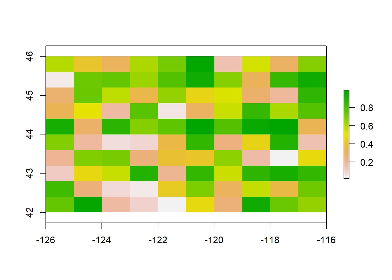
library(raster) r <-raster(ncol=10, nrow =10, xmx=-116,xmn=-126,ymn=42,ymx=46)r
Note that just specifying the number of rows and columns and extent was sufficient to create a RasterLayer object. The number of rows and columns defined our spatial resolution of the raster. In addition, the standard CRS +proj=longlat +datum=WGS84 +no_defs was automatically assigned. At the moment, our raster is empty, i.e. it is simply a grid with no data values. Let us generate some data to populate the raster by assigning random values from the unit distribution to each grid cell.
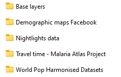
Download the “Geo-spatial Bangladesh data” zip file, unzip it, and save it in your working directory. Your folder structure after unzipping should look like this:
Figure 4.15: Folder structure
We would recommend not rearranging the files across folders. Keeping this structure will make it easy to run your code in Section 3 as you will only need to replace the base Working Directory with your own and everything else should run from there!
Warning
Just a heads up that the files we will be working with are very large. The .zip file itself is is 5GB, while all the files after unzipping will take up around 34GB of space. Please make sure you have sufficient memory on your machine (a minimum of 34 GB will be required). If you are using an online storage solution, you might want to temporarily offload other files you are not currently using to the cloud.