
library(dplyr)
library(readr)
library(sf)
library(raster)
library(haven)
library(ggplot2)9 Estimation
9.1 Using the Fay Herriot model to predict poverty in Bangladesh
9.1.1 Step 1: Gathering your geospatial data
This step of the estimation procedure is the material covered in part 1 of the guide. Ensure to save this dataset to your working directory since it is used throughout the process.
Alternatively, for practice following the remainder of the guide, or to ensure you have followed the steps correctly and your data looks the same, you can download the file BGD.zonal.new.version.csv with pre-processed estimates .
9.1.2 Step 2: Spatial joining of the datasets and then generating direct estimates of poverty and their sampling variances
This step is necessary in order to generate our poverty estimates for the in sample areas. Since the DHS survey employs a sampling strategy we cannot take the values they produce at face-value and first have to adjust them to make them to make them more representative of the whole sample.
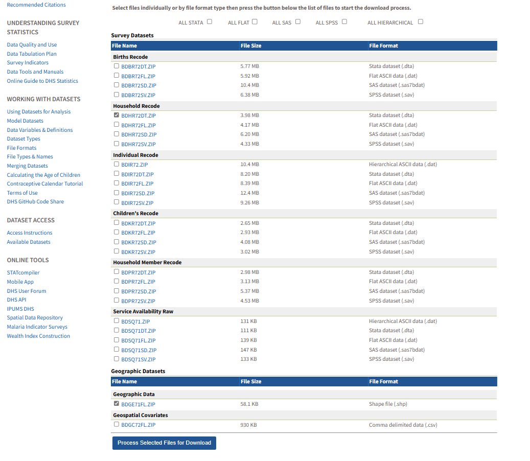
The first step is to download the Bangladesh household poverty data from the DHS website. From this link you will need to click on the 2014 Bangladesh survey. The datasets we are interested are the household recode since this gives the household data on poverty in the country. We are also interested in the Bangladesh shapefile dataset since this gives the co-ordinates of every upazila. We then harmonise these two datasets in order to portray the data on a map. To download these files you will need to register an account with DHS and give a brief explanation of what you intend to do with the data. For this you can explain that you wish to generate spatially disaggregated poverty estimates for the country.
Tip
Top tip: when requesting access to the data, remember to tick the box requesting geospatial data as well!
When applying to the DHS for data they say that they will get back to you with their decision within 2 business days (for us it was just a matter of a couple of hours) but be mindful that you should apply for the data a couple of days before you decide to follow this guide.
We now need to harmonise these two files (the geographic data and the household recode) by doing a spatial join. This generates the unique domain identifier for each observation so that you are able to identify each observation by both its upazila as well as its cluster.
So now you have downloaded the two datasets specified in the screenshot above, we need to merge them together. We start by loading the 2014 DHS Shape file which gives us the GPS coordinates of the centroid of the DHS clusters. We keep only relevant variables from the shapefile so the dataset does not get too large and unwieldy.
# Set working directory
setwd("./data/DHS 2014/BD_2014_DHS_06132023_156_196138/GPS coordinates/DHS HH GPS/BDGE71FL")

# Open the shape file from 2014 DHS data
GPS.DHS.2014 <- st_read("BDGE71FL.shp")

# Get column names
colnames(GPS.DHS.2014)

# Keep only relevant variables - longitude, latitude, geometry, DHS cluster ID
GPS.DHS.2014 <- GPS.DHS.2014[c("DHSCLUST","LATNUM","LONGNUM", "geometry")]
Next we load the DHS Housheold Recode 2014. This dataset contains information on the household wealth index which is what we use to make our variable of interest and this can be merged with the GPS shapefile using the DHS cluster number. We keep the variables: household ID, wealth index, DHS cluster ID, household number, sampling weight and wealth quintile rank as well since these are necessary for us to include in our modelling. We also rename them in order to make the process clearer when using the variables later.
# Set working directory
setwd("./data/DHS 2014/BD_2014_DHS_06132023_156_196138/BDHR72DT")

# Load the 2014 DHS Household recode module
DHS.2014.HH <- read_dta("BDHR72FL.dta")

# Renaming the variables of interest - household ID, wealth index, DHS cluster ID, household number, sampling weight, wealth quintile rank
DHS.2014.HH <- DHS.2014.HH %>% rename("DHSCLUST" = "hv001",
                                      "wealth_quintile_rank"= "hv270",
                                      "hh_sample_weight" = "hv005",
                                      "hh_number" ="hv002",
                                      "wealth_index" = "hv271",
                                      "year" = "hv007",
                                      "strata" = "hv023")
# Keep only the variables of interest as specified above
DHS.2014.HH <- DHS.2014.HH[c("year", "hhid", "DHSCLUST","wealth_index","hh_sample_weight", "hh_number", "wealth_quintile_rank", "strata")]

# Join the DHS household recode with GPS shapefile
DHS.2014.geocoded <- left_join(DHS.2014.HH, GPS.DHS.2014)
We are now able to perform a spatial join to match the household clusters to upazilas. We first use longnum and latnum to turn a data frame with coordinates into a spatial object. We then ensure that the 2 shapefiles have the same projection so that they can be joined without conflict. We then perform a spatial join between the spatial points data frame from DHS and a spatial polygons data frame from the Bangladesh shapefile. This shapefile is the same one you downloaded in section A, step 3 saved as: bgd_admbnda_adm3_bbs_20201113.shp. This function will check whether each spatial point (geographical coordinate) from the DHS shapefile falls inside any polygon from the Bangladesh shapefile and return a data frame with successfully matched information from both spatial objects.
If you are only following section B of the guide and using our pre-loaded harmonised geospatial covariates dataset then you will need to download the shape files here: Bangladesh - Subnational Administrative Boundaries - Humanitarian Data Exchange. You will need to download the zip file entitled bgd_adm_bbs_20201113_SHP.zip.
# Load shapefile

shapefile.zonal <- shapefile("./data/Geo-spatial Bangladesh data/Base layers/admin 3 level/bgd_admbnda_adm3_bbs_20201113.shp")
# Turn data frame into spatial points data frame
coordinates(DHS.2014.geocoded) <- ~LONGNUM+LATNUM

# Set projection as the same for both data frames - based on the projection from the Bangladesh shapefile
proj4string(shapefile.zonal) <- CRS("+proj=longlat +datum=WGS84 +no_defs")
proj4string(DHS.2014.geocoded) <- CRS("+proj=longlat +datum=WGS84 +no_defs")

# Perform the spatial join between the DHS shapefile and the Bangladesh shapefile.
ID <- over(DHS.2014.geocoded, shapefile.zonal)
DHS.2014.geocoded@data <- cbind(DHS.2014.geocoded@data , ID )

# Turn the spatial points data frame into a regular data frame
bgd_dhs_geo_2014 <- as.data.frame(DHS.2014.geocoded)

# Remove the geometry column and null columns for csv formatting
bgd_dhs_geo_2014 <- bgd_dhs_geo_2014[ , -which(names(bgd_dhs_geo_2014) %in% c("geometry" , "ADM3_REF", "ADM3ALT1EN", "ADM3ALT2EN"))]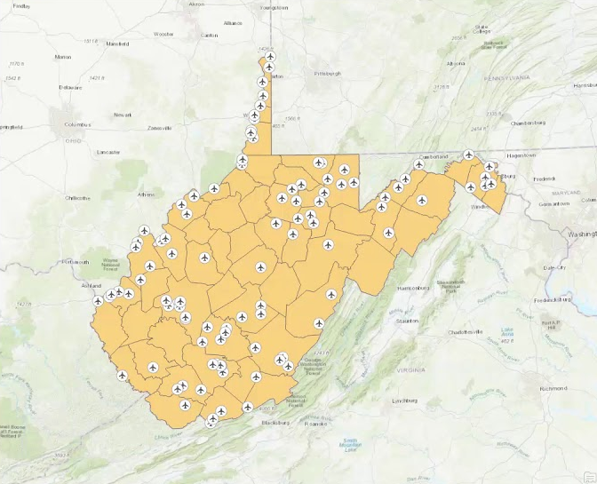
Figure 9.2 showing the location of airfields in West Virginia, is an example of how a spatial join works. The main shapefile has the county lines loaded and the outline of the shape representing the state border. The second shapefile shows every airfield and their respective GPS coordinates. When the two shapefiles are projected in the same perspective a spatial join is then able to tell you in which county the airfield is based. This is the same concept as our study with the spatial join informing us in which upazila each cluster of households is located based on the GPS coordinates.
Once we format the new dataframe correctly and remove the unnecessary columns, the new dataframe is represented by bgd_geo_2014.csv. This dataframe combines the required variables from the household recode module for the 2014 DHS, the geo-location of clusters of households, and upazila codes to which the clusters belong. This dataset we are now using has information on: wealth index raw score, quintile ranking of the wealth index, strata, household weights, upazila, number of clusters and GPS location of clusters.
The GPS coordinates we use correspond to the centroid of a cluster of households, which has a random offset of 2km in urban areas and 5-10km in rural areas to preserve the privacy of households. However, the DHS note that efforts have been made for offsets to be specified in a way that preserves the original administrative units within which HHs reside - therefore this should not affect our matching of households to upazilas.
Our next step is to generate our variable of interest. In our case we are looking to create a poverty map so we will be creating a variable using the wealth index, however, this could easily be adapted to create indicators for other key macroeconomic objectives. We create the variable binary_wealth. This is a binary variable that is set as equal to 1 if the household was defined as being in the lowest quintile of wealth in Bangladesh by the DHS survey. Otherwise the variable is set as equal to 0. By definition 20% of households across the country will be in this bottom quantile but you will be able to see which areas are poorer by seeing which areas across the country have a higher probability of a household being in this bottom quintile of wealth.
We also create a variable to determine how many clusters were sampled in each upazila because depending on this, the estimates will be more or less precise due to the change in sample size. The number of clusters in each upazila is also necessary for our variance estimation in the next stage of the estimation procedure.
Tip
The dataset we use this for this is the bgd_geo_2014.csv dataset we just created in the spatial join so ensure you have this file saved to your working directory!
First you need to install and load necessary packages for the estimation:
library(survey)
library(nlme)
library(emdi)
library(dplyr)
library(sae)
library(MASS)
We then run the code as follows:
# Check how many observations there are there in each cluster
Ban_data <- bgd_dhs_geo_2014 %>%
  group_by(ADM3_PCODE) %>%
  mutate(num_clusters = n_distinct(DHSCLUST))

# Display values in a table
frequency_table <- table(Ban_data$num_clusters)

print(frequency_table)
   1    2    3    4    5   10   12
6139 5858 3105 1269  289  288  352
# Calculating the numbers of clusters per Upazila
upazila_cluster_count <- Ban_data %>%
group_by(ADM3_PCODE) %>%
summarize(num_clusters = n_distinct(DHSCLUST))
# Summarize the count of clusters per Upazila
cluster_summary <- table(upazila_cluster_count$num_clusters)
# View the summary table
print(cluster_summary)
  1   2   3   4   5  10  12
214 101  36  11   2   1   1
# Constructing a binary variable for whether a HH belongs to the lowest wealth quintile.
Ban_data$binary_wealth <- 0
# Replace with 1 if the HH belongs to the lowest quintile
Ban_data$binary_wealth[Ban_data$wealth_quintile_rank == 1] <- 1Now we know how many clusters are in each upazila, we are able to generate the direct estimates and the sampling variances. The method varies if there is only 1 cluster per upazila compared to if there are multiple clusters, since by definition if there is only one cluster in the upazila there will be the same variation in the cluster as in the whole upazila. Therefore,if there is only one upazila in the cluster, we use a design effect. If there is more than 1 cluster in the upazila we are able to calculate using the survey() package.
First of all we calculate the direct estimates and the sampling variances for every upazila using the survey package, regardless of how many clusters are in the area. We set the vartype = "se" rather than confidence intervals because we need the variance later in order to generate the poverty estimates. The second step is that we will then overwrite the direct estimates and variances for the upazilas which have only one cluster using the second method of the design effect.
Direct and standard error estimation for all upazilas (irrespective of the number of clusters)
# Create a survey design object, accounting for household weights, strata, and clusters
DHS.design <- svydesign(ids = ~ DHSCLUST,
                        weights = ~ hh_sample_weight,
                        strata = ~ strata,
                        data = Ban_data)

de <- svyby(~ binary_wealth,
            by = ~ADM3_PCODE,
            design = DHS.design,
            svymean,
            vartype=c("se"))

# Check standard errors
summary(de$se)
Min. 1st Qu. Median Mean 3rd Qu. Max.
0.00000 0.00000 0.00000 0.02097 0.02375 0.21625 We now look at the direct estimates and sampling variances for observations where there is only one cluster in an upazila. We use a design effect to do this. The design effect of a single-stage cluster sample, assuming equal selection probabilities and clusters of size M, is given by design effect (henceforth deff or de) = 1 + (M - 1)* ICC where ICC is the intra-cluster correlation coefficient for the variable of interest. ICC is estimated by the variance of the binary_wealth variable in the cluster divided by the variance of the poorest variable of the cluster added to the variance of the household. The DHS survey design involves a second stage of selection of a group of 30 households out of those in the cluster (113 on average) therefore we have set M = 4.
The design effect is effectively a multiplier that quantifies the impact of a survey design on the variability of estimates. It indicates how much larger the sample size would have to be compared to a simple random sample to achieve the same level of precision as the DHS survey with its complex design. As a result of this, in the modelling procedure later, we divide the number of households per upazila by the design effect in order to calculate the effective sample size per upazila.
We fit the model using the lme function from the package nlme. STRS stands for stratified simple random sampling. We use an lme model (linear mixed effects) since it incorporates both fixed and random effects. This takes into account the overall relationships between variables which are the same for all upazilas in the data (fixed effects), and also takes into account variations in data across different upazilas that are specific to a certain upazila (random effects).
Estimation of design effect for upazilas with one cluster
# Fitting a linear model with just an intercept
fit.rs <- lme(binary_wealth ~ 1,
              random = ~1 |
                DHSCLUST, method = "ML",
                data = Ban_data[Ban_data$num_clusters ==
                                1, ])
# Variance covariance matrix
vcomp <- as.numeric(VarCorr(fit.rs))

# Save this as a matrix
test.matrix <- VarCorr(fit.rs)
test.matrix
DHSCLUST = pdLogChol(1)
Variance StdDev
(Intercept) 0.04473346 0.2115029
Residual 0.13668278 0.3697063# Calculate the design effect
deff.1clus <- 1 + (4 -1) * vcomp[1]/(vcomp[1] + vcomp[2])
# Check design effect
deff.1clus[1] 1.739737# Calculate standard errors
# Create a survey design object for upazilas with just one cluster
design.STSRS <- svydesign(id = ~1,
weights = ~hh_sample_weight,
strata = ~strata,
data = Ban_data)
de.STSRS <- svyby(~binary_wealth,
by = ~ADM3_PCODE,
design = design.STSRS,
svymean,
vartype=c("se"))
de.STSRS <- dplyr::select(de.STSRS,
ADM3_PCODE, se.STSRS = se)
# Create an object with upazila codes and number of clusters
sizes <- Ban_data[, c("num_clusters", "ADM3_PCODE")]
de <- merge(de, sizes,
by = "ADM3_PCODE") %>%
merge(de.STSRS, by = "ADM3_PCODE") %>%
mutate(se.imp = ifelse(num_clusters ==
1, se.STSRS *
sqrt(deff.1clus),
se))
# Remove duplicates
final_de <- de[!duplicated(de$ADM3_PCODE), ]
View(final_de)Pre-smoothing this is what the CV (coefficient of variation) looks like:
#  2. Test our data  #
# Turn number of clusters into factor
final_de$num_clusters_factor <- as.factor(final_de$num_clusters)

# Calculate the coefficient of variation in our data
final_de$cve <- (final_de$se.imp / final_de$binary_wealth)

# Plot
ggplot(final_de, aes(x=binary_wealth, y=cve, color=num_clusters_factor)) + geom_point()
Warning: Removed 67 rows containing missing values (`geom_point()`).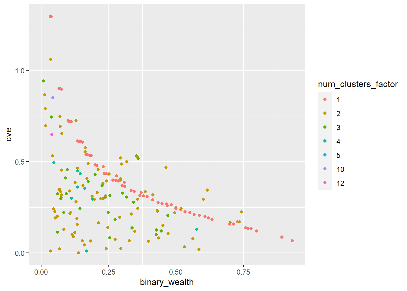
The coefficient of variation is simply calculated as the standard deviation over the mean. A CV of below 20% or 0.2 is often required for publication.
Smoothing the variance estimates using a Generalised Variance Function
To reduce the volatility in the coefficient of variation as seen in the graph above, we use an additional smoothing step that involves the use of Generalised Variance Functions. Smoothing the variance estimates may be needed in order to improve the performance of area-level models. Smoothing involves the initial variance estimates being replaced by corresponding predicted values produced under a linear regression model.
The predictors we use in this model include the direct estimates of our variable of interest ‘binary_wealth’, the square of the direct estimates, the number of clusters representing each upazila, the square of the number of clusters and the average sampling weight for a household in each upazila. In order to avoid undue impact of influential observations, the model is fitted by using only the data of upazilas with fewer than 5 clusters. This is because, as seen in the plot and frequency tables above, there are relatively few upazilas with more than 5 clusters in them so a model estimating standard errors might be overly influenced by large outliers.
The steps of this process are as follows:
Calculate the average HH weight for each upazila
Fit a linear model where the outcome is an estimate of the standard errors and the predictors are: direct estimates of binary_wealth, the square of the direct estimates, the number of clusters representing each upazila, the square of the number of clusters and the average sampling weight for a household in each upazila. This process is done using a subset of the upazilas that have fewer than 5 clusters.
Make a data frame with fitted values from this linear model, upazilas to which those correspond, and the number of clusters.
Replace the original CV (coefficient of variation) by fitted values for upazilas that have 2-4 clusters.
# Calculate the average sampling weight for households in an upazila
Ban_data <- Ban_data %>%
  group_by(ADM3_PCODE) %>%
  mutate(avg_hh_weight = mean(hh_sample_weight))

# Create a data frame with just the average hh weight and upazila code
avg_weight_df <- Ban_data[, c("avg_hh_weight", "ADM3_PCODE")]

# Remove duplicates
avg_weight_df <- avg_weight_df[!duplicated(avg_weight_df$ADM3_PCODE), ]

summary(final_de)
ADM3_PCODE binary_wealth se num_clusters
Length:365 Min. :0.00000 Min. :0.00000 Min. : 1.000
Class :character 1st Qu.:0.03891 1st Qu.:0.00000 1st Qu.: 1.000
Mode :character Median :0.17241 Median :0.00000 Median : 1.000
Mean :0.22012 Mean :0.02097 Mean : 1.636
3rd Qu.:0.34304 3rd Qu.:0.02375 3rd Qu.: 2.000
Max. :0.93103 Max. :0.21625 Max. :12.000
se.STSRS se.imp num_clusters_factor cve
Min. :0.00000 Min. :0.00000 1 :214 Min. :0.0000
1st Qu.:0.03278 1st Qu.:0.01843 2 :101 1st Qu.:0.2253
Median :0.05531 Median :0.06959 3 : 35 Median :0.3635
Mean :0.05071 Mean :0.06576 4 : 11 Mean :0.4309
3rd Qu.:0.07725 3rd Qu.:0.10884 5 : 2 3rd Qu.:0.5368
Max. :0.09619 Max. :0.21625 10: 1 Max. :1.2978
12: 1 NA's :67 # Merge with the final_de data
final_de <- left_join(final_de, avg_weight_df)Joining with `by = join_by(ADM3_PCODE)`# Make a subset for upazilas with fewer than 5 clusters
final_de_subset <- subset(final_de, num_clusters < 5)
# Remove observations where standard errors are 0 (this does not tell us anything about the variability of the estimate since there is no variation)
final_de_subset <- subset(final_de_subset, se.imp > 0)
# Fitting a linear model
model1 <- lm(se.imp ~ binary_wealth + I(binary_wealth^2) + num_clusters + I(num_clusters^2) + avg_hh_weight,
data = final_de_subset, na.action=na.omit)
summary(model1)
Call:
lm(formula = se.imp ~ binary_wealth + I(binary_wealth^2) + num_clusters +
    I(num_clusters^2) + avg_hh_weight, data = final_de_subset,
    na.action = na.omit)

Residuals:
      Min        1Q    Median        3Q       Max
-0.086978 -0.006404  0.000132  0.005862  0.117462

Coefficients:
                     Estimate Std. Error t value Pr(>|t|)
(Intercept)         8.292e-02  9.320e-03   8.897  < 2e-16 ***
binary_wealth       3.524e-01  2.519e-02  13.989  < 2e-16 ***
I(binary_wealth^2) -3.361e-01  3.356e-02 -10.014  < 2e-16 ***
num_clusters       -5.555e-02  9.117e-03  -6.093 3.53e-09 ***
I(num_clusters^2)   9.138e-03  2.131e-03   4.288 2.46e-05 ***
avg_hh_weight      -5.589e-10  1.552e-09  -0.360    0.719
---
Signif. codes:  0 '***' 0.001 '**' 0.01 '*' 0.05 '.' 0.1 ' ' 1

Residual standard error: 0.02616 on 289 degrees of freedom
Multiple R-squared:  0.6016,    Adjusted R-squared:  0.5947
F-statistic: 87.27 on 5 and 289 DF,  p-value: < 2.2e-16
# Save fitted values in a data frame - initial variance estimates should be replaced by predicted values from this model
fitted <- as.data.frame(model1[["fitted.values"]])
summary(fitted) model1[["fitted.values"]]
Min. :0.001596
1st Qu.:0.057203
Median :0.082503
Mean :0.080963
3rd Qu.:0.106662
Max. :0.128517 # Save upazila codes in a list
upazilas <- final_de_subset$ADM3_PCODE
# Add to the fitted data frame
fitted$ADM3_PCODE <- as.character(upazilas)
# Get column names
colnames(fitted)[1] "model1[[\"fitted.values\"]]" "ADM3_PCODE" # Rename column
names(fitted)[names(fitted) == 'model1[["fitted.values"]]'] <- 'se.GVF'
# Have a look
summary(fitted$se.GVF) Min. 1st Qu. Median Mean 3rd Qu. Max.
0.001596 0.057203 0.082503 0.080963 0.106662 0.128517 # Save number of clusters in a list
clusters <- final_de_subset$num_clusters
# Add to the fitted data frame
fitted$num_clusters <- as.numeric(clusters)
# Now look at the summary
summary(fitted$se.GVF) Min. 1st Qu. Median Mean 3rd Qu. Max.
0.001596 0.057203 0.082503 0.080963 0.106662 0.128517 # Left join with final_de dataframe
final_de <- left_join(final_de, fitted)Joining with `by = join_by(ADM3_PCODE, num_clusters)`# Replace NA values of se.GVF with the previous standard errors - this is equivalent to smoothing for all upazilas that have 1-4 clusters
final_de$se.GVF <- ifelse(is.na(final_de$se.GVF), final_de$se.imp, final_de$se.GVF)
# Now re-calculate CV
final_de$cve.2 <- (final_de$se.GVF / final_de$binary_wealth)
# Plot
ggplot(final_de, aes(x=binary_wealth, y=cve.2, color=num_clusters_factor)) + geom_point() Warning: Removed 67 rows containing missing values (`geom_point()`).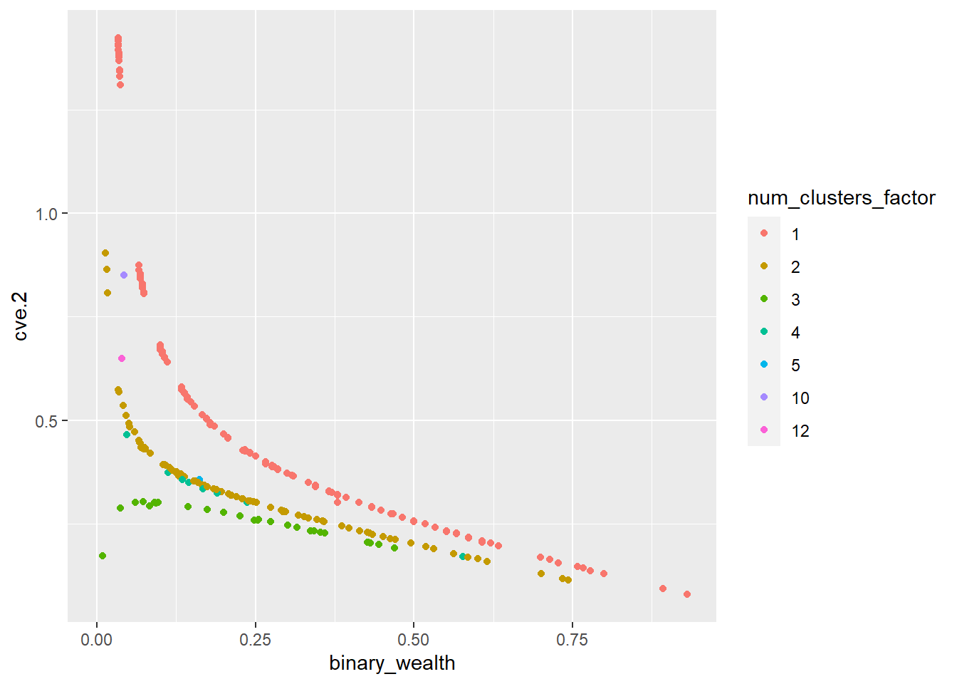
You can see in the graph above that the CV is much smoother and this is much more appropriate when predicting variables using area level models since it reduces noise, stabilizes estimates and enhances model performance. The above model explains 62% of the variability present in the data. After fitting the model, only the variances for upazilas represented with fewer than 5 clusters are smoothed.
Now our datasets that we will use for the FH modelling are ready! We have the final_de dataframe which includes our variable of interest and the standard errors we have estimated using the generalised variance function (se.GVF). The other dataframe is the BGD_zonal_new_version which includes our geospatial variables.
9.1.3 Step 3: How to combine your datasets. Getting your geospatial data and direct estimates of poverty in the same dataframe.
We use the merge command to merge two dataframes together. We then use the column bind command to create the variable new_df$se.GVF^2 which is standard errors squared from the generalised variance function (GVF). This is used as the variable vardir which is an important argument in the FH model.
BGD_zonal_new_version <- read_csv("./data/BGD.zonal.new.version.csv")

View(BGD_zonal_new_version)

# Merging the geospatial data and the household poverty data with updated variance estimation from step 2
new_df <- left_join(BGD_zonal_new_version, final_de)

# Creating new variable with the
new_df = cbind(new_df, new_df$se.GVF^2)

attach(new_df)

View(new_df)
9.1.4 Step 4: Covariate selection for initial model.
This step follows the principle of parsimony in order to slim down the model to find only the geospatial covariates that have the highest predictive power.
To do this we first create a new subsetted dataframe, excluding the variables that were used to create the wealth index or the standard errors of the wealth index. Since these are not geospatial covariates and will clearly be highly correlated with our binary_wealth indicator of interest. We also exclude the upazila.code column since we only want to include the geospatial covariates to see which are the most significant predictors of poverty.
We then fit a full linear regression model using the new dataframe.
# Subset of the dataframe
new_df2 <- new_df[,c(3:165)]

# Fitting a linear regression model
full_model2 <- lm(binary_wealth ~ ., data = new_df2)
We then perform stepwise selection based on BIC criterion to narrow down the number of variables from 150+ to around 15-20. K refers to the number of degrees of freedom used for the penalty, or in other words, how selective the criterion will be when including a variable in the model.
stepwise_model2 <- stepAIC(full_model2, direction = "both", trace = FALSE, k = log(nrow(new_df2)))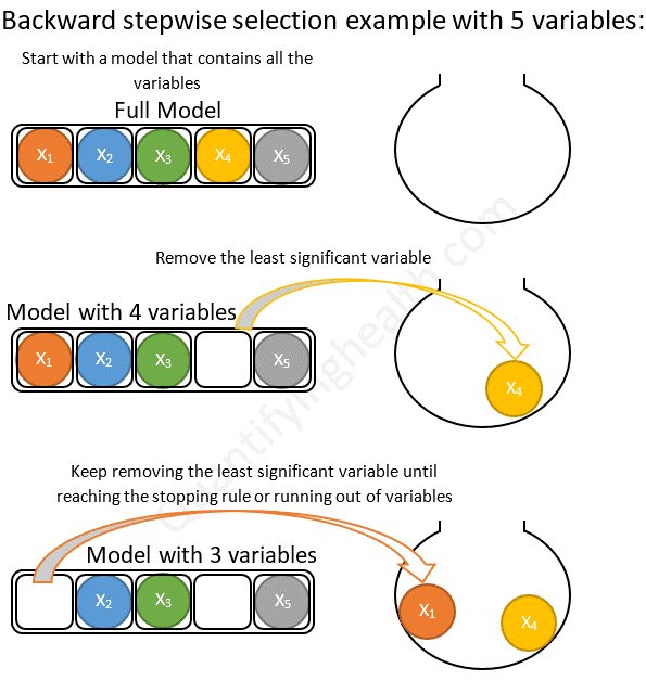
Figure 9.3 is an illustrative example showing how a basic backwards model selection would work. Forward stepwise selection is the same in reverse, it starts with the null model and adds the most significant variables until the stopping criterion is reached. Since we are running a stepwise model it uses both forward and backward steps to iteratively add and remove variables until no further changes need to be made to the model.
We can then view the selected geospatial variables which we will use in our cursory model.
summary(stepwise_model2)
Call:
lm(formula = binary_wealth ~ min.osm_dst_waterway_100m_2016_BGD +
    max.bgd_women_2020 + max.bgd_women_of_reproductive_age_15_49_2020 +
    max.esaccilc_dst_water_100m_2000_2012_BGD + max.esaccilc_dst140_100m_2014_BGD +
    mean.X201501_Global_Travel_Time_to_Cities_BGD + mean.esaccilc_dst_water_100m_2000_2012_BGD +
    mean.esaccilc_dst011_100m_2014_BGD + mean.osm_dst_road_100m_2016_BGD +
    sum.X201501_Global_Travel_Time_to_Cities_BGD + sum.bgd_children_under_five_2020 +
    sum.bgd_general_2020 + sum.bgd_men_2020 + sum.bgd_women_of_reproductive_age_15_49_2020 +
    sum.bgd_youth_15_24_2020 + sum.esaccilc_dst140_100m_2014_BGD +
    sum.osm_dst_road_100m_2016_BGD + sum.Nightlights_data + stdev.esaccilc_dst130_100m_2014_BGD +
    count.X201501_Global_Travel_Time_to_Cities_BGD + count.X202001_Global_Motorized_Travel_Time_to_Healthcare_BGD,
    data = new_df2)

Residuals:
     Min       1Q   Median       3Q      Max
-0.34966 -0.08750 -0.01316  0.07413  0.45352

Coefficients:
                                                               Estimate
(Intercept)                                                   1.858e-01
min.osm_dst_waterway_100m_2016_BGD                            9.970e-03
max.bgd_women_2020                                            1.351e-03
max.bgd_women_of_reproductive_age_15_49_2020                 -2.509e-03
max.esaccilc_dst_water_100m_2000_2012_BGD                    -1.948e-02
max.esaccilc_dst140_100m_2014_BGD                            -4.413e-03
mean.X201501_Global_Travel_Time_to_Cities_BGD                 9.720e-03
mean.esaccilc_dst_water_100m_2000_2012_BGD                    3.296e-02
mean.esaccilc_dst011_100m_2014_BGD                           -2.077e-02
mean.osm_dst_road_100m_2016_BGD                              -4.447e-02
sum.X201501_Global_Travel_Time_to_Cities_BGD                 -1.321e-07
sum.bgd_children_under_five_2020                              2.783e-05
sum.bgd_general_2020                                         -1.449e-05
sum.bgd_men_2020                                              1.532e-05
sum.bgd_women_of_reproductive_age_15_49_2020                  1.815e-05
sum.bgd_youth_15_24_2020                                     -5.131e-06
sum.esaccilc_dst140_100m_2014_BGD                             9.206e-08
sum.osm_dst_road_100m_2016_BGD                                8.284e-07
sum.Nightlights_data                                         -4.967e-06
stdev.esaccilc_dst130_100m_2014_BGD                           2.872e-02
count.X201501_Global_Travel_Time_to_Cities_BGD               -3.399e-04
count.X202001_Global_Motorized_Travel_Time_to_Healthcare_BGD  3.402e-04
                                                             Std. Error t value
(Intercept)                                                   3.881e-02   4.789
min.osm_dst_waterway_100m_2016_BGD                            3.463e-03   2.879
max.bgd_women_2020                                            3.548e-04   3.807
max.bgd_women_of_reproductive_age_15_49_2020                  6.651e-04  -3.772
max.esaccilc_dst_water_100m_2000_2012_BGD                     6.606e-03  -2.949
max.esaccilc_dst140_100m_2014_BGD                             1.411e-03  -3.126
mean.X201501_Global_Travel_Time_to_Cities_BGD                 1.718e-03   5.658
mean.esaccilc_dst_water_100m_2000_2012_BGD                    1.238e-02   2.663
mean.esaccilc_dst011_100m_2014_BGD                            7.124e-03  -2.916
mean.osm_dst_road_100m_2016_BGD                               1.152e-02  -3.861
sum.X201501_Global_Travel_Time_to_Cities_BGD                  2.988e-08  -4.421
sum.bgd_children_under_five_2020                              3.273e-06   8.504
sum.bgd_general_2020                                          1.721e-06  -8.423
sum.bgd_men_2020                                              1.901e-06   8.057
sum.bgd_women_of_reproductive_age_15_49_2020                  3.066e-06   5.919
sum.bgd_youth_15_24_2020                                      1.533e-06  -3.347
sum.esaccilc_dst140_100m_2014_BGD                             3.744e-08   2.459
sum.osm_dst_road_100m_2016_BGD                                2.391e-07   3.464
sum.Nightlights_data                                          1.015e-06  -4.892
stdev.esaccilc_dst130_100m_2014_BGD                           6.116e-03   4.696
count.X201501_Global_Travel_Time_to_Cities_BGD                1.345e-04  -2.527
count.X202001_Global_Motorized_Travel_Time_to_Healthcare_BGD  1.345e-04   2.530
                                                             Pr(>|t|)
(Intercept)                                                  2.50e-06 ***
min.osm_dst_waterway_100m_2016_BGD                           0.004241 **
max.bgd_women_2020                                           0.000167 ***
max.bgd_women_of_reproductive_age_15_49_2020                 0.000190 ***
max.esaccilc_dst_water_100m_2000_2012_BGD                    0.003406 **
max.esaccilc_dst140_100m_2014_BGD                            0.001921 **
mean.X201501_Global_Travel_Time_to_Cities_BGD                3.23e-08 ***
mean.esaccilc_dst_water_100m_2000_2012_BGD                   0.008122 **
mean.esaccilc_dst011_100m_2014_BGD                           0.003781 **
mean.osm_dst_road_100m_2016_BGD                              0.000135 ***
sum.X201501_Global_Travel_Time_to_Cities_BGD                 1.32e-05 ***
sum.bgd_children_under_five_2020                             5.75e-16 ***
sum.bgd_general_2020                                         1.02e-15 ***
sum.bgd_men_2020                                             1.31e-14 ***
sum.bgd_women_of_reproductive_age_15_49_2020                 7.84e-09 ***
sum.bgd_youth_15_24_2020                                     0.000908 ***
sum.esaccilc_dst140_100m_2014_BGD                            0.014435 *
sum.osm_dst_road_100m_2016_BGD                               0.000599 ***
sum.Nightlights_data                                         1.54e-06 ***
stdev.esaccilc_dst130_100m_2014_BGD                          3.84e-06 ***
count.X201501_Global_Travel_Time_to_Cities_BGD               0.011948 *
count.X202001_Global_Motorized_Travel_Time_to_Healthcare_BGD 0.011864 *
---
Signif. codes:  0 '***' 0.001 '**' 0.01 '*' 0.05 '.' 0.1 ' ' 1

Residual standard error: 0.1349 on 343 degrees of freedom
  (179 observations deleted due to missingness)
Multiple R-squared:  0.5959,    Adjusted R-squared:  0.5712
F-statistic: 24.09 on 21 and 343 DF,  p-value: < 2.2e-16
9.1.5 Step 5: Fitting the model
Our first step of fitting the model is running a cursory model. For this we use the variables that were selected to be most significant by the stepwise selection procedure above. We also carry out the estimation with no transformation on a raw scale to see if the model offers reasonable predictive power.
We can then run a couple of model diagnostic regressions to see how the raw scale fits the data and to see if the vital assumptions are satisfied.
Raw scale estimation:
fh_raw_scale <- fh(fixed = binary_wealth ~ min.osm_dst_waterway_100m_2016_BGD +
    max.bgd_women_2020 + max.bgd_women_of_reproductive_age_15_49_2020 +
    max.esaccilc_dst_water_100m_2000_2012_BGD + mean.X201501_Global_Travel_Time_to_Cities_BGD +
    mean.esaccilc_dst_water_100m_2000_2012_BGD + mean.osm_dst_road_100m_2016_BGD +
    sum.X201501_Global_Travel_Time_to_Cities_BGD + sum.bgd_children_under_five_2020 +
    sum.bgd_general_2020 + sum.bgd_men_2020 + sum.bgd_women_of_reproductive_age_15_49_2020 +
    sum.bgd_youth_15_24_2020 + sum.osm_dst_road_100m_2016_BGD +
    sum.Nightlights_data + stdev.esaccilc_dst130_100m_2014_BGD +
    count.X201501_Global_Travel_Time_to_Cities_BGD + count.X202001_Global_Motorized_Travel_Time_to_Healthcare_BGD +
    min.esaccilc_dst150_100m_2014_BGD, vardir = "new_df$se.GVF^2",
          combined_data = new_df, domains = "ADM3_PCODE", method = "ml",
          MSE = TRUE, mse_type = "analytical")

summary(fh_raw_scale)
When looking at the model summary the adjusted R-squared is 0.57. This might seem like reasonable predictive power.
However, we also need to look at normal probability plots of residuals and random errors to see if there is a clear departure from normality.
To do this, we generate 2 output plots showing:
Normal Q-Q plot showing level 1 residuals
Normal Q-Q plot showing the random effects.
There are two plots since we are using an lme so the first plot shows the residuals of the fixed effects and the second plot shows the distribution of random effects. If the plot follows a straight line then it suggests that the residuals/ random effects are normally distributed which is a key assumption in our model.
lev1 = fh_raw_scale$model$real_residuals
lev2 = fh_raw_scale$model$random_effects
qqnorm(lev1) 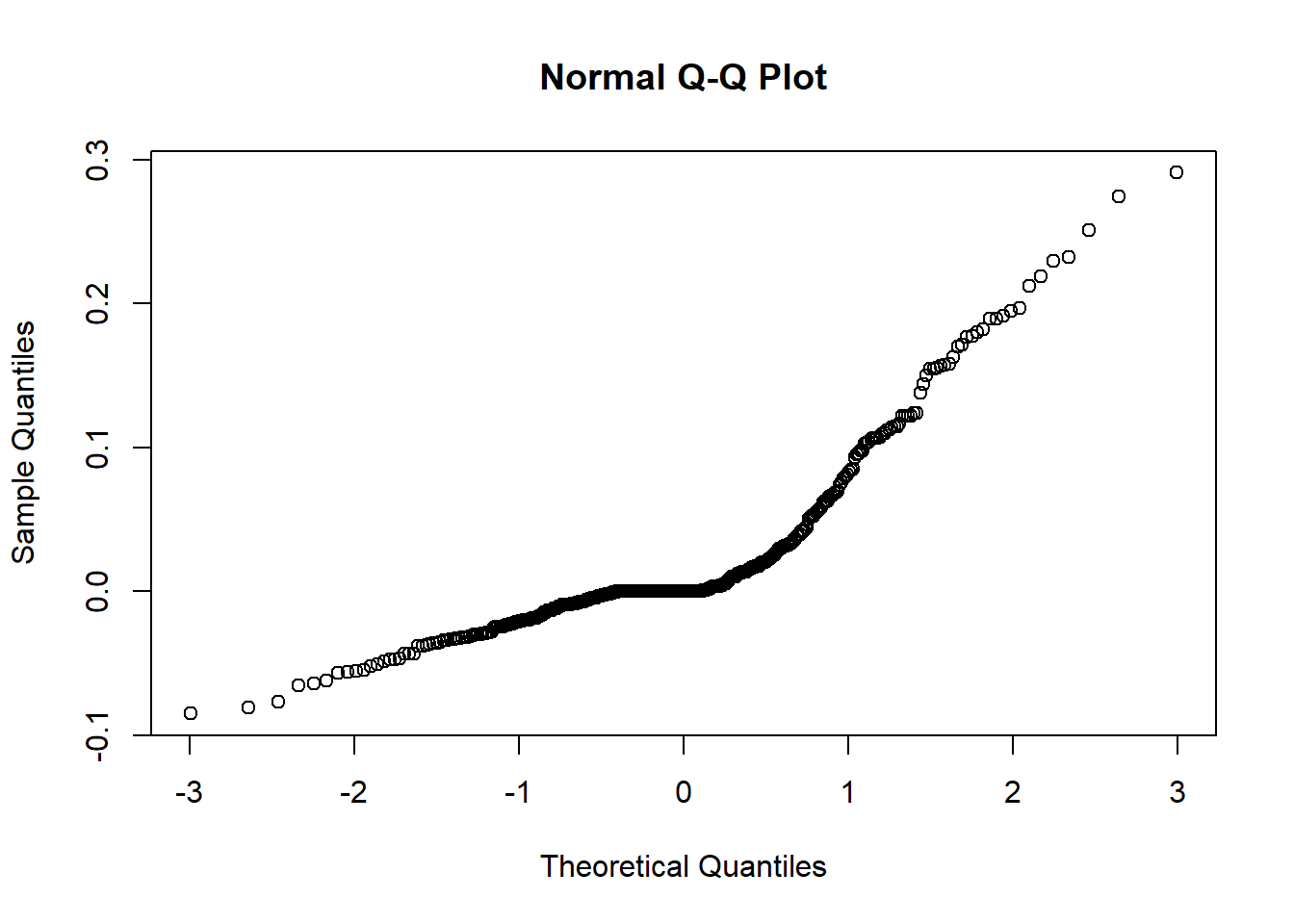
qqnorm(lev2) 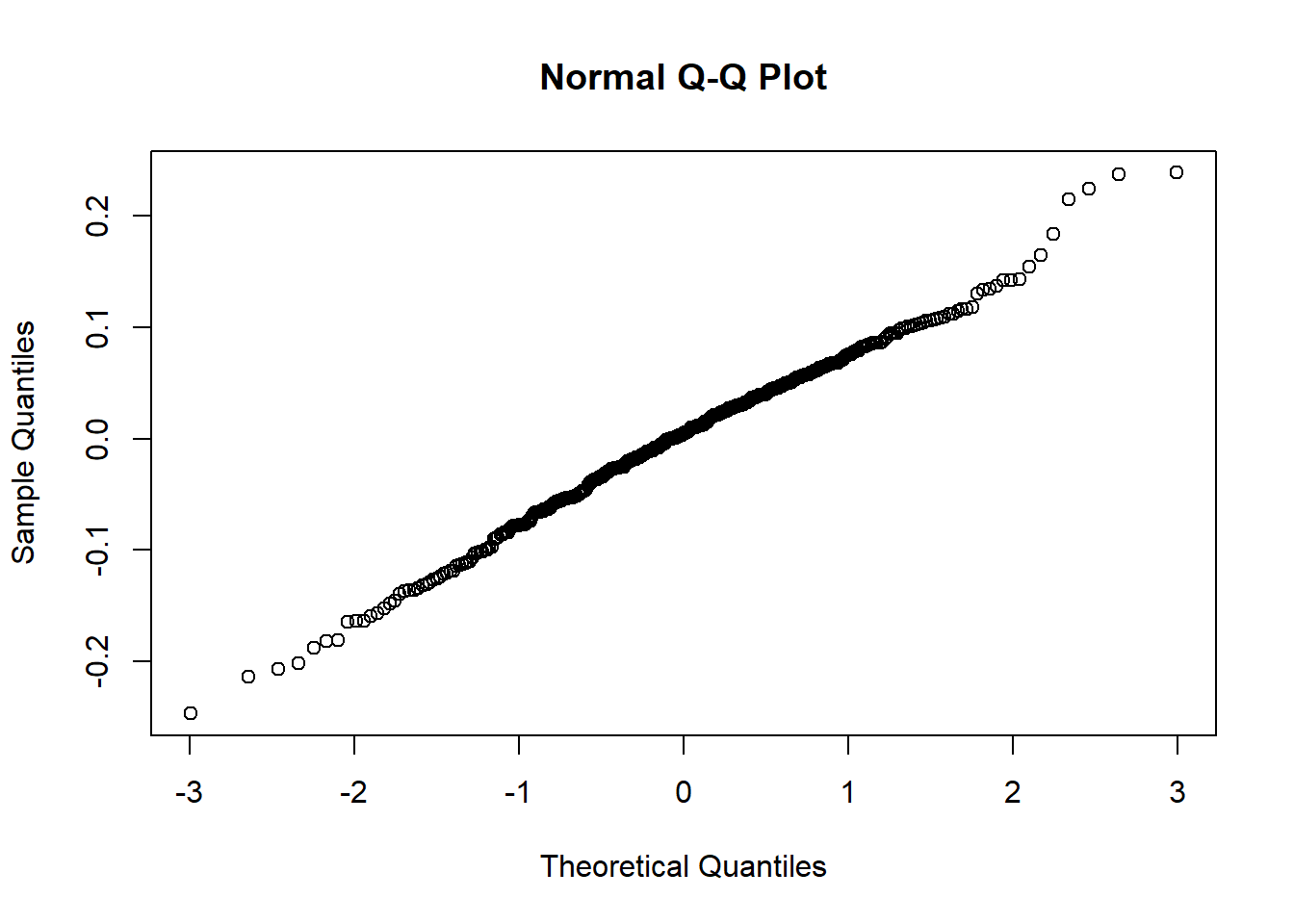
Especially in output plot 1 this graph resembles more of an upwards curve rather than a 45 degree line which we would hope for. This is our first warning sign that potentially the current model is not a great fit for the data.
Therefore, since we are not convinced, we also need to critically evaluate the next diagnostic check. This next function will generate direct and model-based point estimates of our variable of interest binary_wealth as well as corresponding variances and MSEs (mean squared errors). Note that this is only possible if the MSE argument was set equal to TRUE when fitting the area-level model. This second diagnostic model is important to evaluate if we are going to use the model for predictive purposes.
est_raw = estimators(fh_raw_scale, MSE = TRUE)
summary(fh_raw_scale$ind$FH)
Min. 1st Qu. Median Mean 3rd Qu. Max.
-2.19329 0.06146 0.17241 0.18211 0.29282 0.89286 We notice that the model-based point estimates include negative predicted values (min = -2.19) for our variable of interest despite the fact that we are modelling a proportion that obviously should be between 0 and 1. This is a consequence of using a model that does not fit well and illustrates the importance of using model diagnostics.
As a result, in order for the model to better fit the data we are going to try using an arcsin transformation. The arcsin transformation is often used when data is in the form of percentages or proportions that are close to either 0 or 1. The transformation stabilizes the variance of data that follows a binomial distribution, especially when the proportions are close to the boundaries of 0 or 1, as is the case here since binary_wealth is a variable indicating the percentage or proportion of households in each area that are in poverty. Using this transformation requires additional arguments, namely the effective sample size which, as discussed earlier, is defined by the sample size divided by the design effect, as well as the type of backtransformation.
First of all, in order to do this, we need to generate the argument relating to the effective sample size. To do this you first calculate how many households have been surveyed in each upazila from the initial DHS survey. You then load the design effect that we calculated in step 2. The number of households per upazila is then divided by the design effect in order to calculate the effective sample size.
You can then merge this with the new_df we are using to make sure we have all these variables in one dataset.
# Calculating the number of households surveyed per upazila
bgd_geo_2014 <- bgd_dhs_geo_2014 %>%
  group_by(ADM3_PCODE) %>%
  mutate(num_unique_hhid = n_distinct(hhid)) %>%
  ungroup()

# Creating a new variable that represents effective sample size. This is the number of households surveyed per upazila divided by the design effect which we calculated in step 2.
bgd_geo_2014$num_hh_deff <- bgd_geo_2014$num_unique_hhid / deff.1clus


# Merging these new variables with the dataset we are using for the FH model
new_df <- left_join(new_df, bgd_geo_2014)

cleaned_df <- distinct(new_df, ADM3_PCODE, .keep_all = TRUE)
Now we estimate an initial model using the arcsin transformation discussed above whilst still using the geospatial variables which were selected by an initial AIC/BIC variable selection.
fh_arcsin <- fh(fixed = binary_wealth ~ min.osm_dst_waterway_100m_2016_BGD +
    max.bgd_women_2020 + max.bgd_women_of_reproductive_age_15_49_2020 +
    max.esaccilc_dst_water_100m_2000_2012_BGD + mean.X201501_Global_Travel_Time_to_Cities_BGD +
    mean.esaccilc_dst_water_100m_2000_2012_BGD + mean.osm_dst_road_100m_2016_BGD +
    sum.X201501_Global_Travel_Time_to_Cities_BGD + sum.bgd_children_under_five_2020 +
    sum.bgd_general_2020 + sum.bgd_men_2020 + sum.bgd_women_of_reproductive_age_15_49_2020 +
    sum.bgd_youth_15_24_2020 + sum.osm_dst_road_100m_2016_BGD +
    sum.Nightlights_data + stdev.esaccilc_dst130_100m_2014_BGD +
    count.X201501_Global_Travel_Time_to_Cities_BGD + count.X202001_Global_Motorized_Travel_Time_to_Healthcare_BGD +
    min.esaccilc_dst150_100m_2014_BGD, vardir = "new_df$se.GVF^2",
          combined_data = cleaned_df, domains = "ADM3_PCODE", method = "ml",transformation = "arcsin", backtransformation = "bc", eff_smpsize = "num_hh_deff",
          MSE = FALSE, mse_type = "boot", B = 50)

summary(fh_arcsin)
We have initially have set MSE = FALSE above to in order to speed the model stepwise selection step up (the next step) but we will be changing MSE back to true in step 6 when we compute the out of sample estimates.
lev1 = fh_arcsin$model$real_residuals
lev2 = fh_arcsin$model$random_effects
qqnorm(lev1) 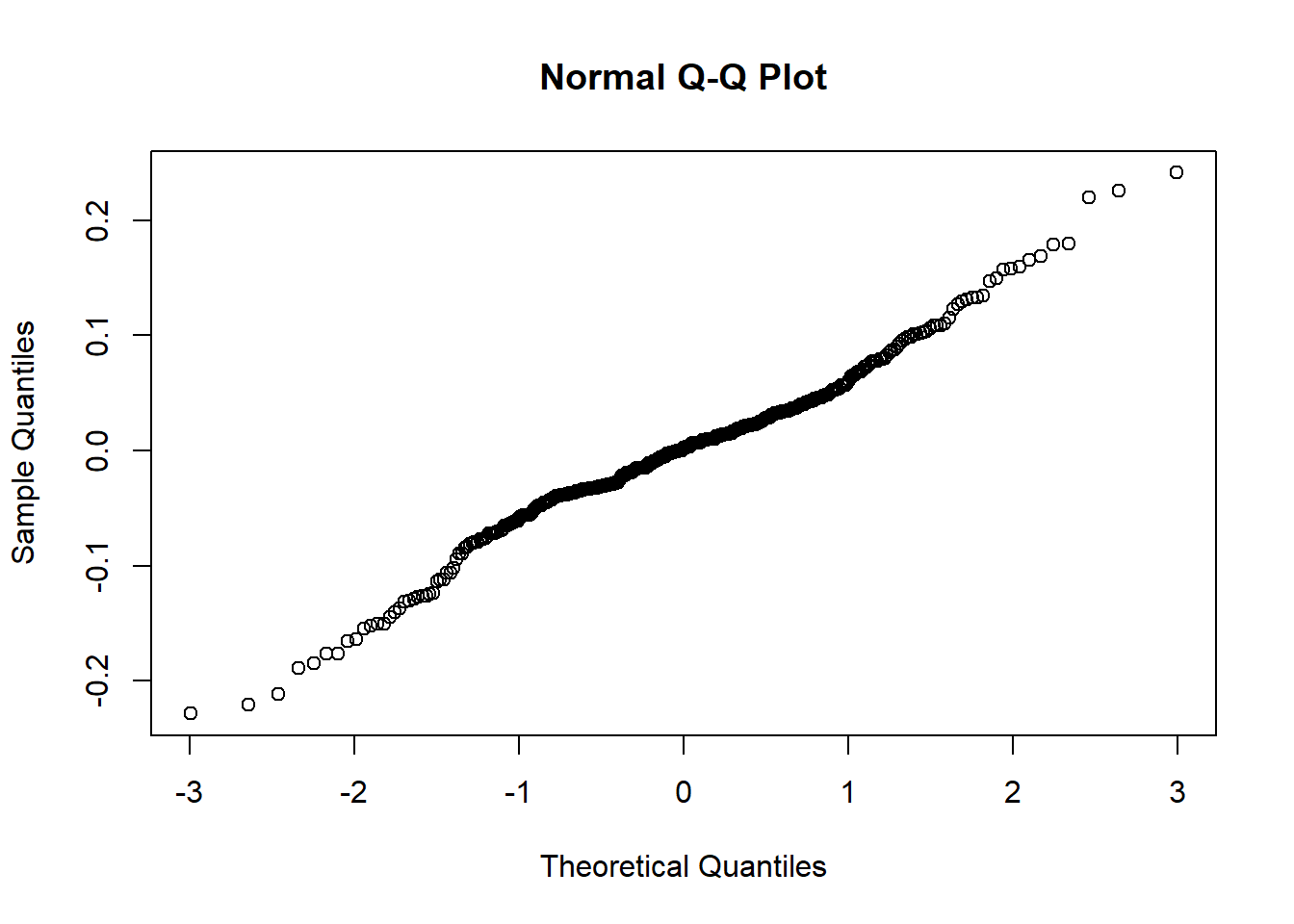
qqnorm(lev2) 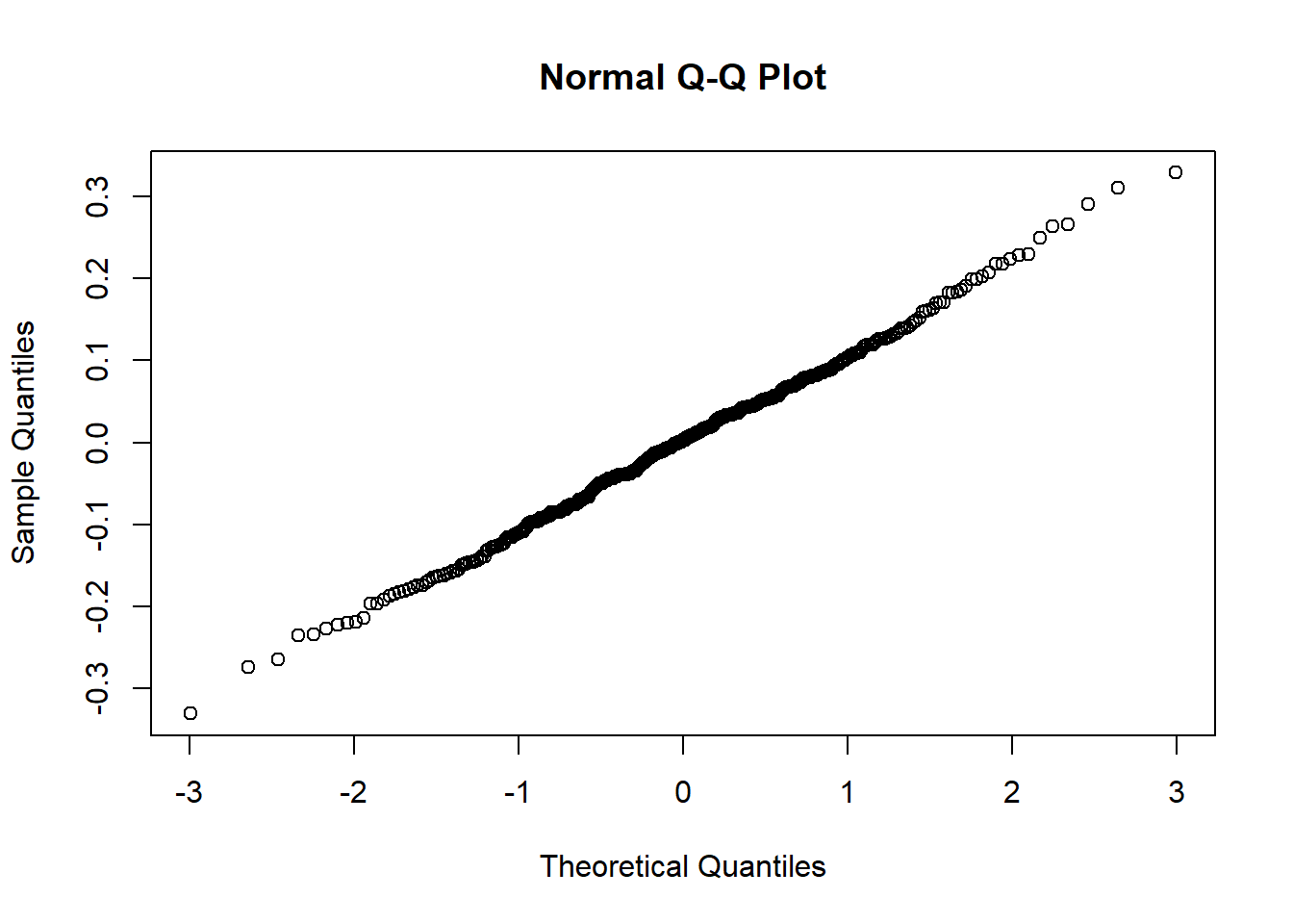
summary(fh_arcsin$ind$FH) Min. 1st Qu. Median Mean 3rd Qu. Max.
0.0000006 0.0636107 0.1718347 0.2096746 0.3067485 0.9247274 Now we can see that both Q-Q plots have close to linear 45 degree relationships. Furthermore, when looking at the second diagnostic model, the range of estimates for the variable binary_wealth is between 0 and 1 which is much more appropriate for a proportion. The mean is close to the value of 0.2 which also makes sense since the variable is calculated by the number of households in the bottom quintile of wealth in the country. Note this may not be exactly equal to 0.2 since population could vary between upazilas and this is just the average of all values without any weighting to take account of population. Now we are satisfied that this transformation satisfies the model assumptions we can carry on with the remaining modelling steps.
We now use the step function again, this time using the BIC criterion to see if additional variables can be dropped from the model. This is again following the principle of parsimony to prevent overfitting when the model begins to do out of sample prediction.
Tip
This step may take a long time to estimate so be patient!
step(fh_arcsin, criteria = "BIC") We then use the variables that are left by this selection process to create our final arcsin model. This is the model we use to produce our out of sample estimates of poverty.
9.1.6 Step 6: FH model prediction for out of sample estimates
After following the previous step and dropping the geospatial covariates as suggested by the stepwise selection above, we are left with the following model.
fh_arcsin_final <- fh(fixed = binary_wealth ~ min.osm_dst_waterway_100m_2016_BGD +      max.bgd_women_2020 + max.bgd_women_of_reproductive_age_15_49_2020 +      max.esaccilc_dst_water_100m_2000_2012_BGD + mean.X201501_Global_Travel_Time_to_Cities_BGD +      mean.esaccilc_dst_water_100m_2000_2012_BGD + mean.osm_dst_road_100m_2016_BGD +      sum.X201501_Global_Travel_Time_to_Cities_BGD + sum.bgd_children_under_five_2020 +      sum.bgd_general_2020 + sum.bgd_men_2020 + sum.bgd_women_of_reproductive_age_15_49_2020 +      sum.bgd_youth_15_24_2020 + sum.osm_dst_road_100m_2016_BGD +      sum.Nightlights_data + stdev.esaccilc_dst130_100m_2014_BGD +      count.X202001_Global_Motorized_Travel_Time_to_Healthcare_BGD +      min.esaccilc_dst150_100m_2014_BGD, vardir = "new_df$se.GVF^2",      combined_data = cleaned_df, domains = "ADM3_PCODE", method = "ml",      transformation = "arcsin", backtransformation = "bc", eff_smpsize = "num_hh_deff",      MSE = TRUE, mse_type = "boot", B = 50)
summary(fh_arcsin_final)
We use 50 bootstraps here but in a real case study you may want to use 200 or even 250. We have also now set the MSE as true since we are going to be using this model for out of sample prediction.
The summary includes a lot of useful information. It also now gives the adjusted R-squared as 0.61. This shows the transformed model is an improvement compared to the raw model.
We now estimate the model-based point estimates again.
est = estimators(fh_arcsin_final)
summary(est$ind$FH)
Min. 1st Qu. Median Mean 3rd Qu. Max.
0.0000011 0.0633058 0.1710392 0.2104303 0.3082658 0.9364516 Unlike earlier, this estimation now shows that there are no negative predicted estimates of the variable of interest binary_wealth.
We now show graphically the results of this estimation to also graphically show that the model fit is sufficient and the assumptions are satisfied. This function gives 4 output plots to help show that the normality assumption has not been violated. The four plots are as follows:
Normal Q-Q plot of standardized residuals.
Normal Q-Q plot of random effects
Kernel densities of distribution of standardized residuals. We want these next two to be close to the standard normal distribution.
Kernel densities of distribution of random effects.
We want the plots 1 and 2 to be as close to a 45 degree line as possible to show normality of the errors for both fixed and random effects. Plots 3 and 4 will hopefully resemble bell curves. If both plots resemble the normal distribution then it provides further evidence that assumptions of normality for both residuals and the random effects are met.
plot(fh_arcsin_final)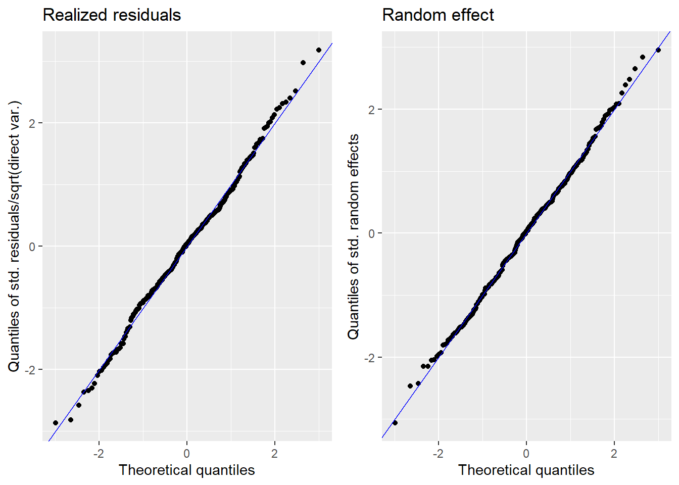
Press [enter] to continue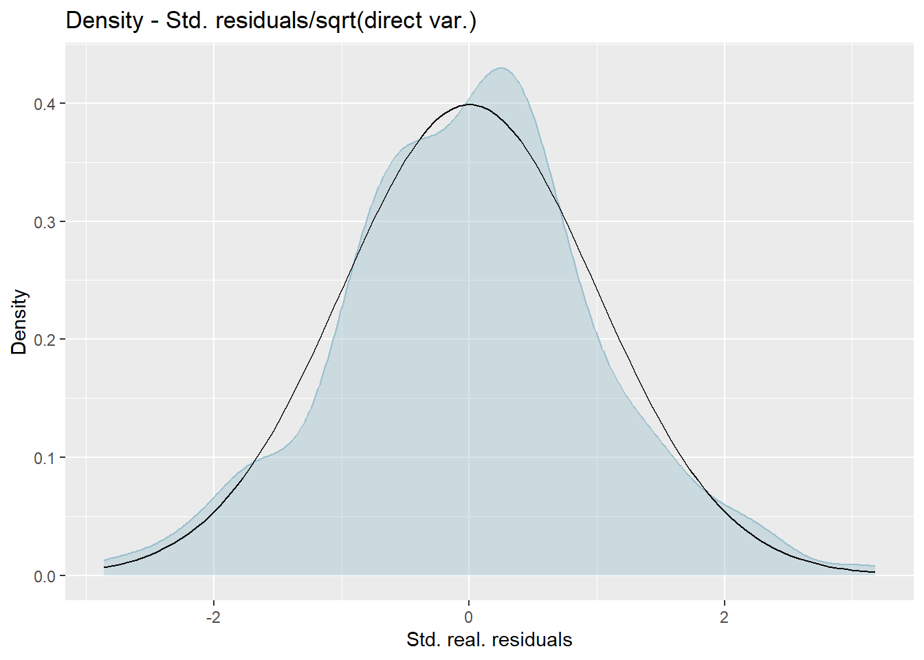
Press [enter] to continue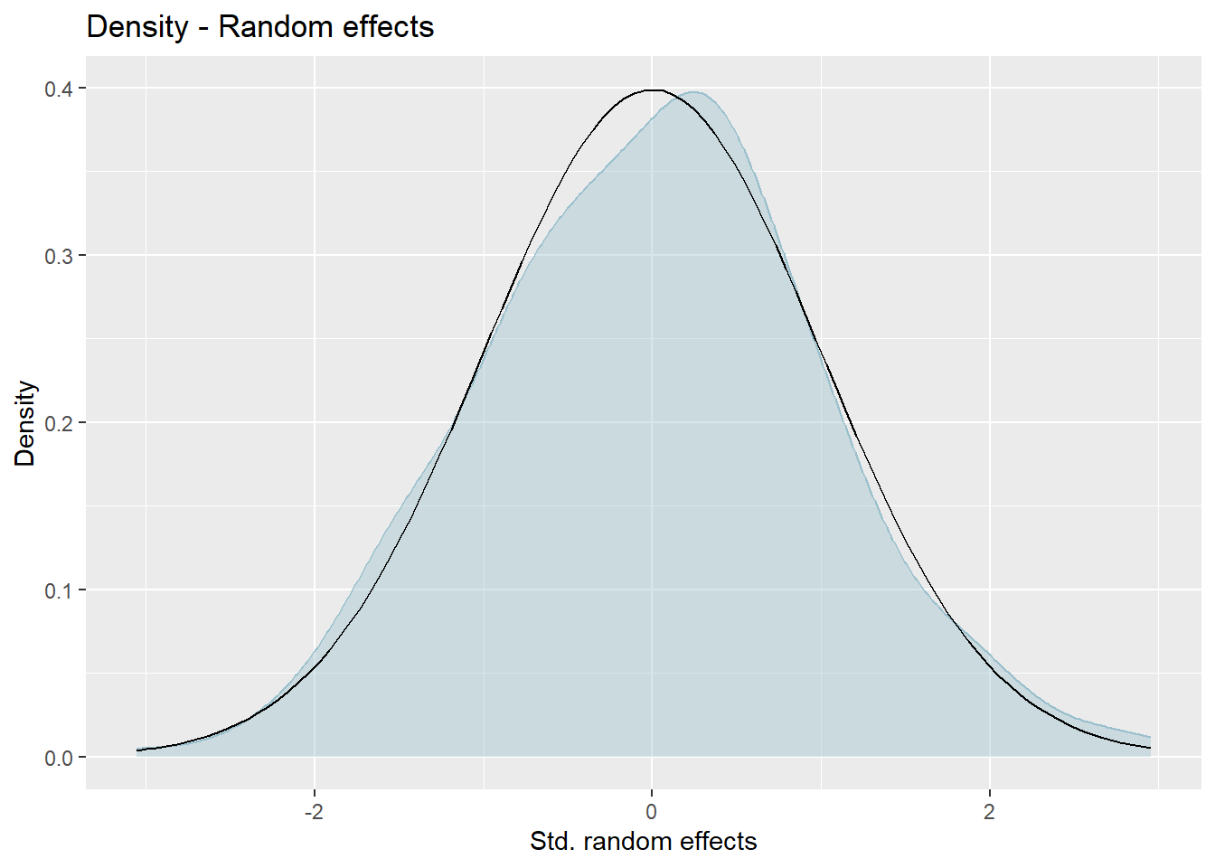
9.1.7 Step 7: Comparison between direct estimates and model estimates
Ideally, model-based point estimates and variances should be consistent with the direct estimates from the survey and their respective variances which we calculated in step 2. We should also expect that the use of model-based methods will produce estimates with improved precision compared to direct estimates.
This command gives the first 6 results just so you can get a general impression that there is an improved precision when using FH estimates vs direct estimates but the values are also very similar. We are also able to see that for domain 302602, which was out of sample in the DHS survey (hence the NA), we now have estimates for the variable ‘binary_wealth’ through using the FH model!
head(estimators(fh_arcsin_final, MSE = TRUE)) Domain Direct Direct_MSE FH FH_MSE
1 BD404104 0.0000000 0.000000000 0.031197853 0.003258623
2 BD302602 NA NA 0.007327699 0.001590023
3 BD501006 NA NA 0.222259686 0.011268381
4 BD555202 0.2934528 0.006799816 0.279989645 0.003288456
5 BD100602 0.2068966 0.008981170 0.171190996 0.003811441
6 BD603602 NA NA 0.345463450 0.016613487We are now also able to graphically compare direct estimates to model based estimates by using the plot command.
The plots below compare the direct estimates against the model-based point estimates. The results show that model-based estimates are correlated well with direct estimates.
compare_plot(fh_arcsin_final) Please note that since all of the comparisons need a direct estimator, the plots are only created for in-sample domains.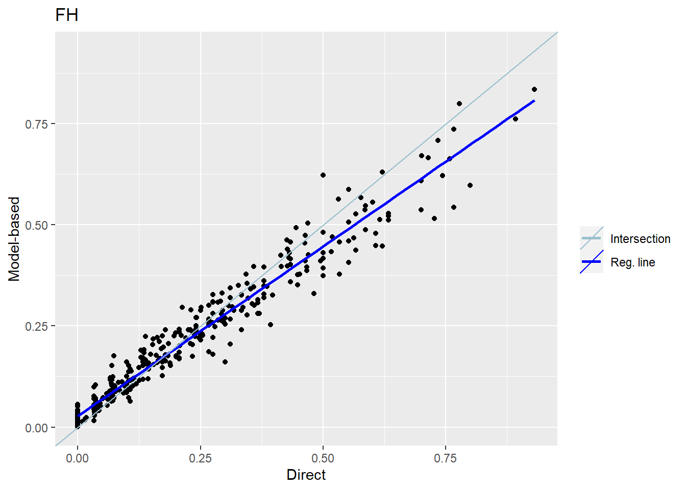
Press [enter] to continue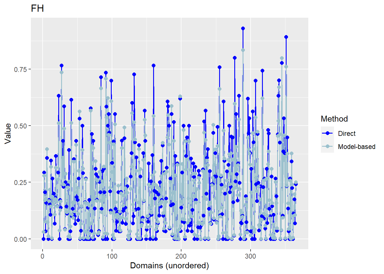
Despite this relationship passing the ‘eye-test’ we then also carry out a Brown test to test this relationship computationally. This command carries out a Brown test to test the Null hypothesis that EBLUP estimates do not differ significantly from the direct estimates
compare(fh_arcsin_final)Please note that the computation of both test statistics is only based on in-sample domains.Brown test
Null hypothesis: EBLUP estimates do not differ significantly from the
direct estimates
W.value Df p.value
73.14329 365 1
Correlation between synthetic part and direct estimator: 0.78 The output of this command shows that the correlation between the two sets of point estimates is 0.73. In addition, this command performs a statistical test on the differences between the direct and model-based point estimates. The p-value of the test is 1 indicating that the null hypothesis of no difference between the two sets of estimates is not rejected.
Benchmark the estimates here if required
This is useful for statistical offices if they want estimates to sum to official figures for reporting.
9.1.8 Step 8: Visualising the results on administrative level 3 (Upazila) scale:
Congratulations! We have now finished generating the poverty estimates using the FH model and all that is left is to display this information on a beautiful map!
First install and load necessary packages
library(ggplot2)
library(ggmap)
library(scales)
library(RColorBrewer)
library(maps)
library(sf)
library(mapproj)
Now we create a new variable named est which includes the both direct and FH estimates from our final model as selected above.
est = estimators(fh_arcsin_final, MSE = FALSE)
attach(est)
We now set our working directory to where we have downloaded our Bangladesh administrative level 3 shape file and download it to R. This shapefile is the same as what we used in step 3 of section A of the guide as well as section B step 2.
setwd("./data/Geo-spatial Bangladesh data/Base layers/admin 3 level")
# Reading Bangladesh shapefile at administrative level 3
bgd_admin3 <- st_read("bgd_admbnda_adm3_bbs_20201113.shp")
extent(bgd_admin3)
The extent command is a quick check to show the minimum and maximum x and y coordinates that the shapefile contains.
We create a new object using the est estimators and renaming the Domain column as ADM3_PCODE in order to match column names in the shapefile.
est.maps <- data.frame(est) %>% mutate(ADM3_PCODE = Domain)We now just need to merge the shape file with the data frame which includes both the direct and FH estimates
est.shp.coef <- left_join(bgd_admin3, est.maps)Map of direct estimates
The commands for creating the maps of direct estimates vs FH estimates are almost identical. To create the visualisation for the direct estimates you use the argument fill = Direct, compared to fill = FH for the FH estimates. You are also able to adjust the title of this map under the name argument, technically the estimation is showing the probability a household in that upazila is in the bottom quintile of wealth distribution across the country. You are also easily able to adjust the scale of the plot, for example setting pretty_breaks(n=10) if you want the scale at 0.1 (1/10) intervals of probability instead of what it is currently set at 0.2 (1/5).
ggplot() + geom_sf(data=est.shp.coef, aes(fill=Direct), color="black", linewidth= 0.25) + theme_nothing(legend = TRUE) + scale_fill_distiller(name = "Proportion of Households in Poverty", palette = "Greens", direction = 1, breaks = pretty_breaks(n = 5))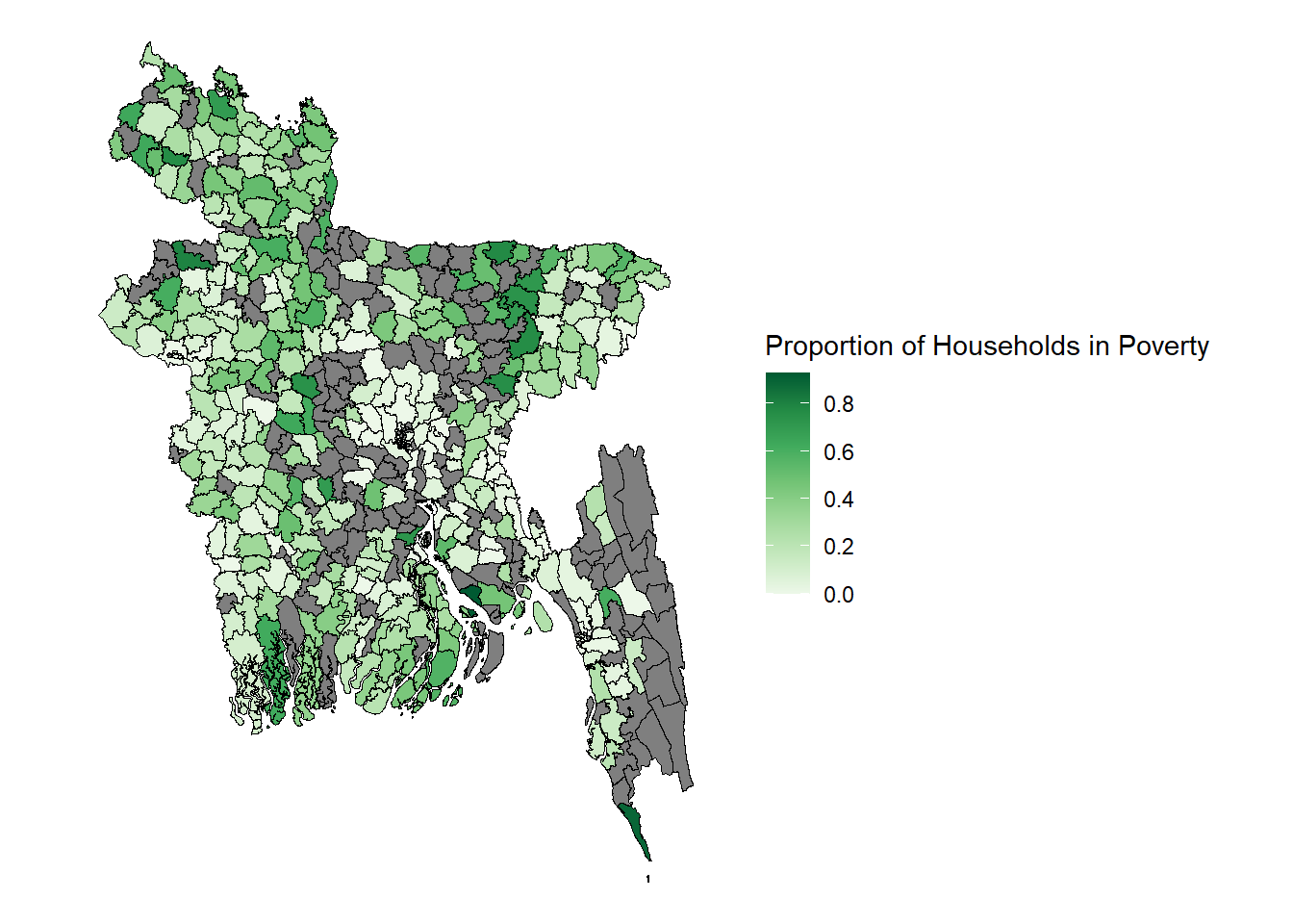
When you look at this map you can clearly see the 179 out of sample areas represented by the regions in grey.
Map of FH estimates
To create the visualisation for the FH estimates you use the argument fill = FH
ggplot() + geom_sf(data=est.shp.coef, aes(fill=FH), color="black", linewidth= 0.25) + theme_nothing(legend = TRUE) + scale_fill_distiller(name = "Proportion of Households in Poverty", palette = "Greens", direction = 1, breaks = pretty_breaks(n = 5))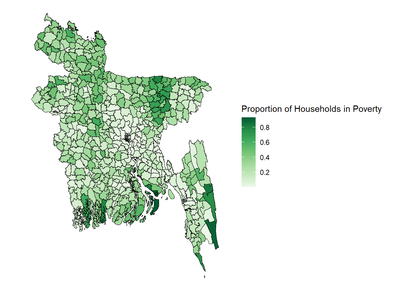
Here all the previously out of sample areas in grey are now shown with their poverty rates as estimated by the Fay-Herriot model. The FH model has used the most statistically significant geospatial covariates to fit a model using data from the DHS household survey as a ground-truth measure of poverty to then predict poverty for out-of-sample areas.
9.1.9 Exporting the results to your medium of choice
If, in addition to the visualisations, you want the raw data for further analysis then it is very easy to export the data to an Excel file. You can then carry out further data-processing on your medium of choice. This command will export the model summary as well as direct and model-based point and uncertainty estimates. The file will be saved in your working directory.
# Exporting estimates to an excel file
write.excel(fh_arcsin_final,             file = "fh_arcsin.xlsx",             MSE = TRUE)