
7 Introduction
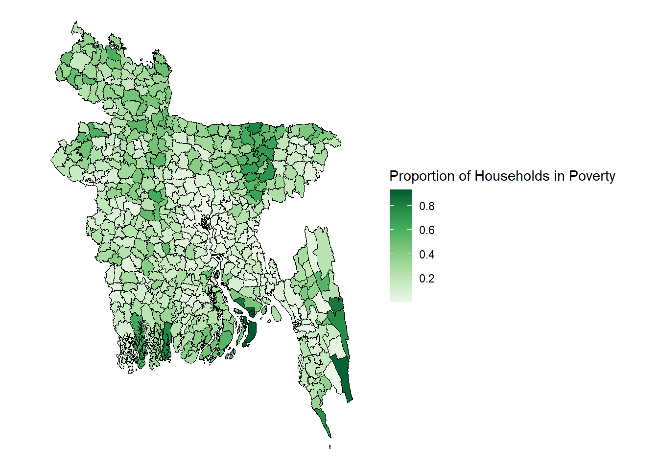
Section A of the guide showed you how to gather and harmonise geospatial data from online in order to make it into a single dataframe ready for analysis. However, as a reminder, the complete estimation procedure of the Fay-Herriot model is an 8 step process! Section B will explain to you how you go from the geospatial dataset you have produced in the first section of the guide, to producing poverty estimates for every upazila in Bangladesh and displaying this information on a map like the one seen in Figure 7.1 below!
The complete steps of the estimation procedure are as follows:
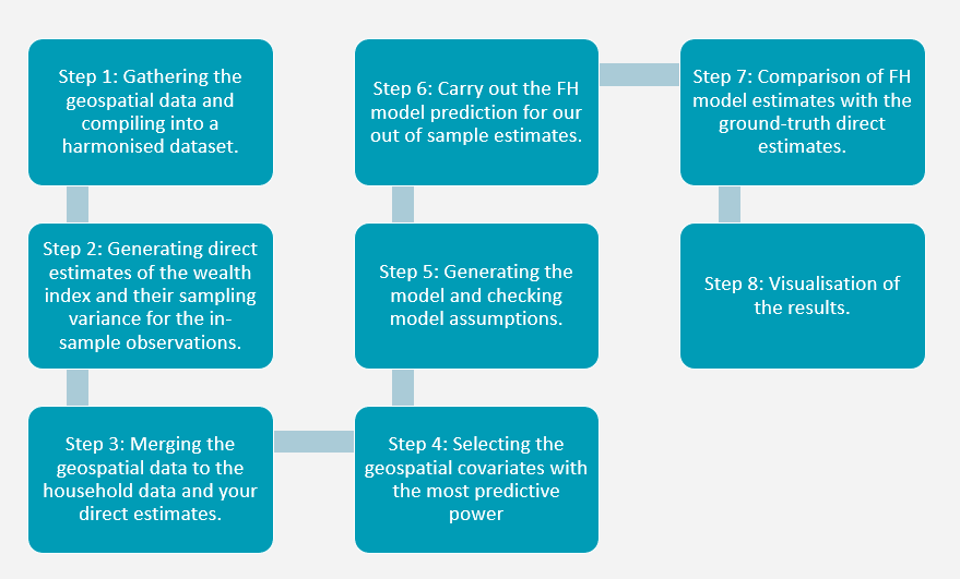
Step 1: Gathering the geospatial data and compiling it into a harmonised dataset.
You can either start with the geospatial co-ordinates you generated in section A, or, if you just want to practice the estimation procedure, you are able to download our pre-processed dataframe BGD.zonal.new.version.csv. Section A of our guide explains how to compile this geospatial dataframe in detail.
Step 2: Carrying out a spatial join of the datasets and then generating direct estimates of poverty and their sampling variance for the in-sample observations.
Our first step here is carrying out a spatial join. Each cluster of households in the DHS survey is uniquely identified but we do not know which upazila they reside within. In order to solve this issue, we overlay the distribution of clusters over a shapefile of the whole country and assign upazila codes to the cluster depending on which polygon they reside within.
Then, in order to account for the fact that surveys often employ complex sampling designs, with elements of stratification and multistage sampling with unequal probabilities, we need to calculate direct estimates of our variable of interest (in our case this is poverty) and estimates of their variances. This is in order to prevent bias being introduced into the estimation. We carry out this step using household wealth data downloaded from the DHS survey.
Once we generate the direct estimates and their variances. We then smooth the variances using a generalised variance function. This improves performance of an area-level model by reducing noise, stablising estimates as well as accounting for uncertainty in the data because of the limited sample size which is an inherent problem when doing prediction using area-level models.
Step 3: Merging the geospatial data to the direct estimates of poverty generated in step 2.
Now we need to combine the geospatial data from section A of the guide and the direct estimates and their variances that you generated in step 2 of the process. In order to combine this information into one big dataset we need a unique common identifier and for this we merge the observations using the unique domain identifier ‘upazila.code’. This code uniquely identifies every single administrative level 3 (upazila level) area in Bangladesh so that R knows which area you are referring to when looking at the values of household poverty and the geospatial covariates. This also is the area code we use later to merge the dataset with the shapefile in order to display our poverty estimates on a map!
Step 4: Selecting the geospatial covariates with the most predictive power
The initial large dataframe we generated in section A with over 150 geospatial variables is unwieldy and following the ‘principle of parsimony’ we want fewer variables. In order to prevent issues such as overfitting we initially trim the model to include fewer covariates. For this we use a selection criterion (AIC/BIC/KIC) to find only the geospatial covariates with the highest predictive power on predicting the variable of interest.
We perform a BIC stepwise selection criterion using all of the available geospatial covariates to see which 15-20 variables perform the best in predicting poverty rates in an area.
Step 5: Generating the model and checking model assumptions.
We now use the geospatial covariates selected in step 4 by the selection criterion in a basic model on a raw scale in order to test the key assumptions of the model and assess the predictive power. For example, the model assumes normality of the error terms which, if violated, introduces bias into the estimation so it is necessary to show that all the necessary assumptions hold.
If the assumptions do not hold with the model in its current format then it is important to carry out a transformation on the target variable. For example log transformations are traditionally popular with income data in order to mitigate issues such as skewed data. In our case, since we are modelling a proportion or a percentage, we use an arcsin transformation. This kind of transformation is common for dealing with data that is bounded between 0 and 1 and is very effective at stabilising the variance of data that follows a binomial distribution.
We then use a variety of visual aids such as plots as well as regression tests to ensure that we are satisfied that all our assumptions hold after a transformation.
Step 6: Carry out the FH model prediction for our out of sample estimates.
In this step we carry out the FH modelling procedure using the model we have developed above that satisfies our assumptions, in order to generate our out of sample wealth estimates. The FH model adopts a bootstrap approach in order to predict out of sample estimates. This is an iterative resampling method which provides estimates of variability and uncertainty without requiring strong assumptions about the data distribution.
The FH model has been trained on in-sample domains which have both geospatial and household data available. However, by definition, only geospatial data is available in out-of-sample domains. By learning the relationship between the most significant geospatial covariates and the variable of interest (as determined by the selection criterion in step 4), the model can estimate what the probability is that a household is in poverty would be in an area that has not been surveyed in the DHS.
Step 7: Comparison of FH model estimates and variances with the ground-truth direct estimates and variances from step 2.
In this step we compare the direct point poverty estimates we generated in step 2 using the DHS data with the FH model estimates that we generated in step 6. This is done both graphically and with a Brown test. This gives some indication of the precision of the model. If we are satisfied with the similarity of the estimates, we can move on to the final stage.
Step 8: Visualisation of the results.
The final step of the process is visualising the results. To do this we use the main Bangladesh shapefile again which includes the co-ordinates of the country’s border lines and includes the polygon shapes for each upazila. We combine this shapefile with our dataset using the unique upazila district code and then visualise the relative wealth in each domain by using a gradient colour scheme.