5 Applying this

In Section 4 we covered key concepts in geo-spatial analysis, including the sources of such data, most common structures, data manipulation and types of spatial objects you might encounter in R. In this section we are going to apply this to a practical problem: we will prepare the geo-spatial covariates (on accessibility, nightlights, topograhy, and demography) that will be used for poverty estimation in Section B. Recall that there are two main types of geo-spatial data: vector and raster. We will primarily be working with raster data and performing what we will call a “harmonisation” - that is, bringing all the rasters to the same extent, shape, spatial resolution, and projection as the base raster layer. Let’s begin with exploring the data sources we will use in this exercise.

5.1 Data sources - Bangladesh

We will be working with the following data sets:

Base layer: WorldPop Administrative Level 0 mastergrid base layer for Bangladesh at ~100m spatial resolution. This mastergrid defines the administrative boundaries of the country, to which we will be harmonising all other geo-spatial datasets, i.e. matching the spatial resolution, CRS, extent, and shape.
Shape file: Subnational Administrative Boundaries for Bangladesh from the Humanitarian Data Exchange. This file contains the administrative boundaries of the zones for which we will be estimating poverty. In our case, this is done at administrative level 3 (upazila) in Bangladesh.
Malaria Atlas data on accessibility, including: travel time to cities and healthcare facilities.
Demographic maps from Meta at ~30m spatial resolution raster showing population density of different demographic groups (men, women, youth, elderly etc.).
Nightlights data at ~450m spatial resolution with almost global coverage.
World Pop Pre-harmonised geo-spatial datasets: available for all countries. The datasets includes information on topography (this relates to land cover classes - for instance, waterways, forests, mountains, plains ets.), slope (measure of change in elevation), and Open Street Map’s data on distance to closest road, waterway. Note that this data has already been harmonised to our base layer and hence will not require any processing in this script.

The below tables provide details on these data sets.

5.1.1 Base layers

Geo-spatial file name	Description	Year	Link to download
bgd_level0_100m_2000_2020.tif	WorldPop Administrative Level 0 mastergrid base layer for Bangladesh	2020	World Pop Hub - National boundarie
bgd_admbnda_adm3_bbs_20201113.shp	Administrative Level 3 (Upazila) Units in Bangladesh	2015	Bangladesh - Subnational Administrative Boundaries - Humanitarian Data Exchange

5.1.2 Geo-spatial data sets to be harmonised

Geo-spatial data
Geo-spatial file name	Description	Year	Link to download
SVDNB_npp_20150101-20151231_75N060E_vcm-orm_v10_c201701311200.avg_rade9.tif	VIIRS night-time lights (global)	2015	Earth Observation Group
2015_accessibility_to_cities_v1.0.tif	MAP travel time to high-density urban centres (global)	2015	Malaria Atlas - Accessibility to Cities
2020_motorized_travel_time_to_healthcare.tif	MAP motorised only travel time to healthcare facilities (global)	2019	Malaria Atlas - Motorised Time Travel to Healthcare
2020_walking_only_travel_time_to_healthcare.tif	MAP walking only travel time to healthcare facilities (global)	2019	Malaria Atlas - Walking Only Time Travel to Healthcare
bgd_general_2020.tif	Meta (Facebook) Population density – Overall; BGD	2020	Humanitarian Data Exchange - Demographic Maps from Meta
bgd_men_2020.tif	Meta (Facebook) Population density – Men; BGD	2020
bgd_elderly_60_plus_2020.tif	Meta (Facebook) Population density – Elderly (aged 60+); BGD	2020
bgd_women_of_reproductive_age_15_49_2020.tif	Meta (Facebook) Population density – Women of reproductive age (15-49); BGD	2020
bgd_women_2020.tif	Meta (Facebook) Population density – Women; BGD	2020
bgd_youth_15_24_2020.tif	Meta (Facebook) Population density – Youths aged 15-24; BGD for 2020	2020
bgd_children_under_five_2020.tif	Meta (Facebook) Population density – Children under 5; BGD	2020

5.1.3 WorldPop harmonised geo-spatial data sets

WorldPop harmonised data
Geo-spatial File Name	Description	Year	Link to Download
bgd_srtm_topo_100m.tif	SRTM topography in BGD	2000	World Pop
bgd_srtm_slope_100m.tif	SRTM slope (derivative of topography) in BGD	2000
bgd_esaccilc_dst040_100m_2014.tif	Distance to ESA-CCI-LC woody-tree area edges in BGD	2014
bgd_esaccilc_dst140_100m_2014.tif	Distance to ESA-CCI-LC herbaceous area edges in BGD	2014
bgd_osm_dst_road_100m_2016.tif	Distance to OSM major roads in BGD	2016
bgd_esaccilc_dst150_100m_2014.tif	Distance to ESA-CCI-LC sparse vegetation area edges in BGD	2014
bgd_osm_dst_roadintersec_100m_2016.tif	Distance to OSM major road intersections in BGD	2016
bgd_esaccilc_dst160_100m_2014.tif	Distance to ESA-CCI-LC aquatic vegetation area edges in BGD	2014
bgd_osm_dst_waterway_100m_2016.tif	Distance to OSM waterways in BGD	2016
bgd_esaccilc_dst190_100m_2014.tif	Distance to ESA-CCI-LC artificial surface edges in BGD	2014
bgd_esaccilc_dst011_100m_2014.tif	Distance to ESA-CCI-LC cultivated area edges in BGD	2014
bgd_esaccilc_dst200_100m_2014.tif	Distance to ESA-CCI-LC bare area edges in BGD	2014
bgd_esaccilc_dst_water_100m_2000_2012.tif	Distance to ESA-CCI-LC inland water in BGD	2012
bgd_wdpa_dst_cat1_100m_2014.tif	Distance to IUCN strict nature reserve and wilderness area edges in BGD	2014
bgd_esaccilc_dst130_100m_2014.tif	Distance to ESA-CCI-LC shrub area edges in BGD	2014
bgd_dst_coastline_100m_2000_2020.tif	Distance to open water coastline in BGD	2000-2020

5.2 Libraries

Throughout this workflow, we will be using functions from the packages shown in the chunk below. Most of them allow for manipulation of spatial objects in R, others are used to enhance our data visualisations. All the below packages need to be installed and loaded in order for the workflow to run smoothly. If you don’t already have some of the below packages installed, you can do so by running: install.packages(“your.package.name”). After that, you will be able to load the package using library(“the.package.you.just.installed”). See below the dependencies we will need for this workflow:

library("tiff")           # opening geoTIFF files
library("raster")         # raster manipulation
library("sf")             # Simple Features vector data
library("ggplot2")        # plots
library("RColorBrewer")   # funky graph colors 
library("haven")          # opening stata files
library("gsubfn")         # string operations
library("viridis")        # colour palette for data visualisations
library("sp")             # Spatial Points vector data
library("plyr")           # Data wrangling
library("dplyr")          # Data wrangling
library("readr")          # read rectangular data
library("leaflet")        # Interactive maps
library("htmlwidgets")    # HTML widgets
library("scales")         # Nice scales on graphs
library("exactextractr")  # Automated production of zonal statistics
library ("cividis")       # Colour palette for data visualisations

5.3 Step 1 - Load all data sets

Our first step will simply be loading all the datasets that we will work with into our environment. The only step that the user needs to complete here is to specify the working directory where the .zip file “Geo-spatial Bangladesh data.zip” is saved (and unzipped). As a reminder, your folder structure should look like this after unzipping:

If this looks right, you are ready to run your first chunk of code below. This will load all the data we will need for this exercise into your environment. Whenever a .tif extension is used, we will import the file and convert it to a raster (recall this is the main format we will be working with). Some folders will have multiple files saved inside them (for example, there are three datasets from the Malaria Atlas Project). In this case, the code will pull all the files that have a .tif extension and save them in a list - so no need to import them individually!

# Set working directory - this is the base folder where we keep all the sub-folders with geo-spatial data organised by source. 
setwd("./data/Geo-spatial Bangladesh data/")

# 1. Base layer #

# Load the WordPop Administrative Level 0 mastergrid base layer for Bangladesh 
base.layer <- 'Base layers/bgd_level0_100m_2000_2020.tif'
base.layer.raster=raster(base.layer)

# 2. Shapefile with boundaries of zones #

# Load the shapefile in a format that's nicer for plotting 
shapefile.zone.plot <- st_read("Base layers/admin 3 level/bgd_admbnda_adm3_bbs_20201113.shp")

# 3. Malaria Atlas accessibility datasets #

#Make a list of all TIFF files from the Malaria Atlas Project and import those into a list 
matlas.list <- list.files(path="Travel time - Malaria Atlas Project", pattern =".tiff", full.names=TRUE)

# Turn all files into a raster and make a list of rasters
matlas.rasters <- lapply(matlas.list, raster)

# 4. Demographic maps from Meta #

# Pull all TIFF files from Meta with demographic maps
fb.list <- list.files(path="Demographic maps Facebook/", pattern =".tif", full.names=TRUE)

# Turn all files into a raster and make a list of rasters
fb.rasters <- lapply(fb.list, raster)

# 5. Nightlights Data #

# Import geoTIFF file on nightlights intensity
nightlights <- 'Nightlights data/SVDNB_npp_20150101-20151231_75N060E_vcm-orm_v10_c201701311200.avg_rade9.tif'

# Turn into a raster 
nightlights.raster = raster(nightlights)

# 6. Pre-harmonised World Pop datasets #

# Make a list of all TIFF files from WorldPop and import those into a list 
worldpop.list <- list.files(path="World Pop Harmonised Datasets", pattern =".tif", full.names=TRUE)

# Turn all files into a raster and make a list of rasters
worldpop.rasters <- lapply(worldpop.list, raster)

You should now be able to view all the data in your environment. Most objects are of the class RasterLayer. Let’s have a closer look at how these objects are structured in practice and the information they contain by inspecting our base layer.

5.3.1 Check the attributes of the base layer

As we will be harmonising all other datasets to our base layer, it is important to understand its attributes. Simply typing the name of our base layer raster object in the console will provide information on: class, dimensions, resolution, extent, crs, source, and names. At the end of the workflow, all of our geo-spatial covariates will have the same spatial resolution, CRS, extent, and shape as our base layer.

# Check attributes associated with the base layer 
base.layer.raster

class      : RasterLayer 
dimensions : 7272, 5596, 40694112  (nrow, ncol, ncell)
resolution : 0.0008333333, 0.0008333333  (x, y)
extent     : 88.01042, 92.67375, 20.57458, 26.63458  (xmin, xmax, ymin, ymax)
crs        : +proj=longlat +datum=WGS84 +no_defs 
source     : bgd_level0_100m_2000_2020.tif 
names      : bgd_level0_100m_2000_2020

# Plot raster
plot(base.layer.raster, box=F, axes=F,legend=F, main = "Bangladesh base layer")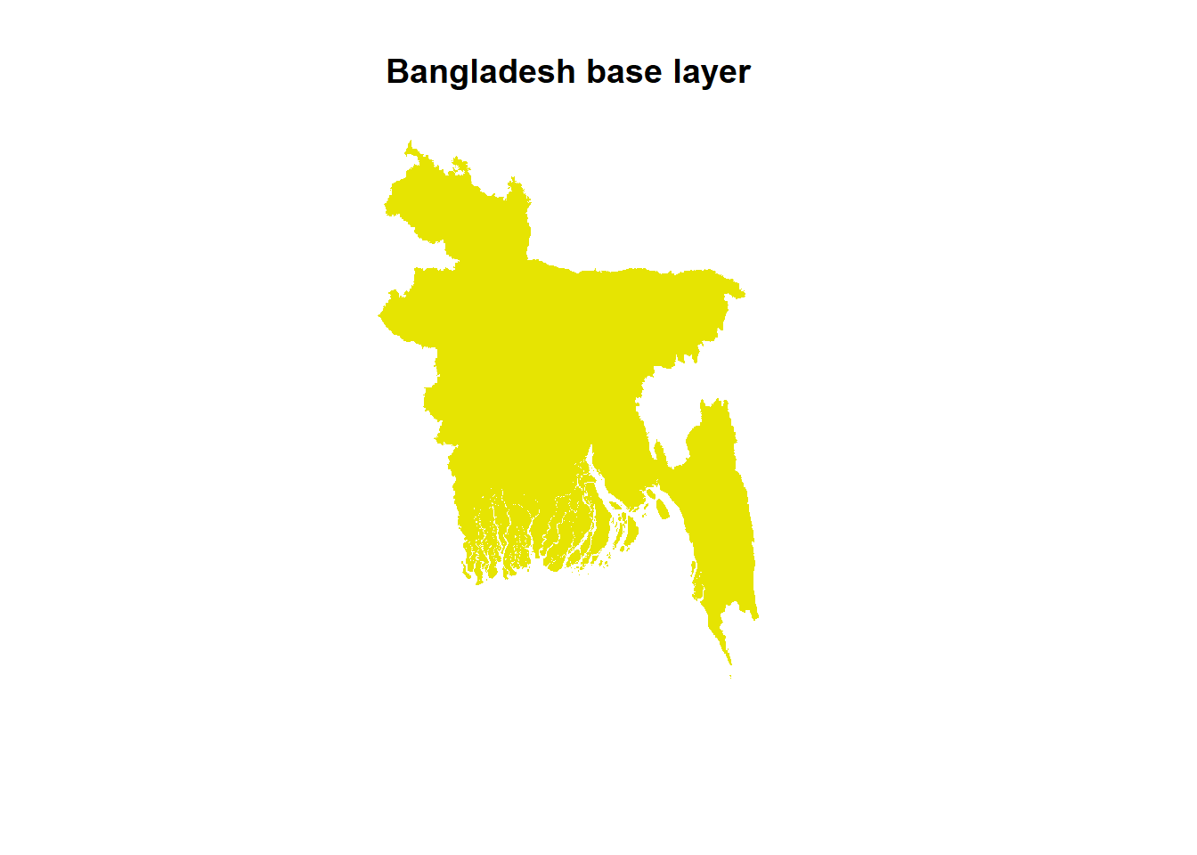

The output is telling us that our object of interest is a RasterLayer, with the following characteristics:

7272 rows, 5596 columns, and 40694112 cells altogether - these are the dimensions of our grid.
A spatial resolution of 0.0008333333 by 0.0008333333 (in degrees). This is equivalent to ~ 100m spatial resolution and defines the size of each cell in the raster.
Extent, i.e. the maximum and minimum values of longitude and latitude which define Bangladesh.
The WGS 1984 datum (EPSG: 4326) geographical projection - this is the most standard global projection.
It came from the GeoTIFF file named “bgd_level0_100m_2000_2020.tif” in our working directory and is named after that file.

We also produced our first map of Bangladesh! This is the raster layer we will be harmonising all our other data to. Note that since this layer simply gives us the administrative national boundaries of Bangladesh, it does not contain any data values. While most of our objects are raster data, we will use one vector dataset: a shapefile containing the boundaries of administrative level 3 (upazilas) in Bangladesh. There are multiple ways of storing vector data in R - let’s have a look.

5.3.2 Inspect the attributes of the shapefile with administrative level 3

Apart from the raster file defining the national boundaries of Bangladesh, we are interested to know the boundaries of the administrative zones that we will estimate poverty for. In our case, this is administrative level 3, or upazila, in Bangladesh. This information is provided by a shapefile, which is a vector dataset - and has different properties than raster data.

As before, we will start by simply typing the name of our spatial object into the console. This will provide information on: geometry, dimensions, extent, CRS, as well as give us a preview into the features. To demonstrate this, we save our shapefile as an sf object with multipolygon geometry.

# Inspect the sf multipolygon object with admin 3 boundaries
shapefile.zone.plot

Simple feature collection with 544 features and 16 fields
Geometry type: MULTIPOLYGON
Dimension:     XY
Bounding box:  xmin: 88.00863 ymin: 20.59061 xmax: 92.68031 ymax: 26.63451
Geodetic CRS:  WGS 84
First 10 features:
   Shape_Leng   Shape_Area    ADM3_EN ADM3_PCODE ADM3_REF ADM3ALT1EN ADM3ALT2EN
1  1.17187865 0.0217530363 Abhaynagar   BD404104     <NA>       <NA>       <NA>
2  0.06885957 0.0002026128     Adabor   BD302602     <NA>       <NA>       <NA>
3  1.23372204 0.0154567631  Adamdighi   BD501006     <NA>       <NA>       <NA>
4  1.03202450 0.0178153322   Aditmari   BD555202     <NA>       <NA>       <NA>
5  0.68737816 0.0137435611 Agailjhara   BD100602     <NA>       <NA>       <NA>
6  1.10900786 0.0164370166 Ajmiriganj   BD603602     <NA>       <NA>       <NA>
7  0.67416928 0.0081541686    Akhaura   BD201202     <NA>       <NA>       <NA>
8  0.75704781 0.0126081808   Akkelpur   BD503813     <NA>       <NA>       <NA>
9  1.09247375 0.0323690689  Alamdanga   BD401807     <NA>       <NA>       <NA>
10 0.77798085 0.0116631673  Alfadanga   BD302903     <NA>       <NA>       <NA>
         ADM2_EN ADM2_PCODE    ADM1_EN ADM1_PCODE    ADM0_EN ADM0_PCODE
1        Jessore     BD4041     Khulna       BD40 Bangladesh         BD
2          Dhaka     BD3026      Dhaka       BD30 Bangladesh         BD
3          Bogra     BD5010   Rajshahi       BD50 Bangladesh         BD
4    Lalmonirhat     BD5552    Rangpur       BD55 Bangladesh         BD
5        Barisal     BD1006    Barisal       BD10 Bangladesh         BD
6       Habiganj     BD6036     Sylhet       BD60 Bangladesh         BD
7  Brahamanbaria     BD2012 Chittagong       BD20 Bangladesh         BD
8      Joypurhat     BD5038   Rajshahi       BD50 Bangladesh         BD
9      Chuadanga     BD4018     Khulna       BD40 Bangladesh         BD
10      Faridpur     BD3029      Dhaka       BD30 Bangladesh         BD
         date    validOn validTo                       geometry
1  2015-01-01 2020-11-13    <NA> MULTIPOLYGON (((89.44292 23...
2  2015-01-01 2020-11-13    <NA> MULTIPOLYGON (((90.35181 23...
3  2015-01-01 2020-11-13    <NA> MULTIPOLYGON (((89.08198 24...
4  2015-01-01 2020-11-13    <NA> MULTIPOLYGON (((89.42583 26...
5  2015-01-01 2020-11-13    <NA> MULTIPOLYGON (((90.17736 23...
6  2015-01-01 2020-11-13    <NA> MULTIPOLYGON (((91.33541 24...
7  2015-01-01 2020-11-13    <NA> MULTIPOLYGON (((91.24459 23...
8  2015-01-01 2020-11-13    <NA> MULTIPOLYGON (((89.02462 25...
9  2015-01-01 2020-11-13    <NA> MULTIPOLYGON (((88.91292 23...
10 2015-01-01 2020-11-13    <NA> MULTIPOLYGON (((89.61672 23...

# Plot the shape file - this shows the zones for which we will estimate poverty
ggplot() + 
  geom_sf(data = shapefile.zone.plot, size = 3, color = "black", fill = "cyan1") + 
  ggtitle("Administrative Level 3 Bangladesh") + 
  coord_sf() + theme_minimal()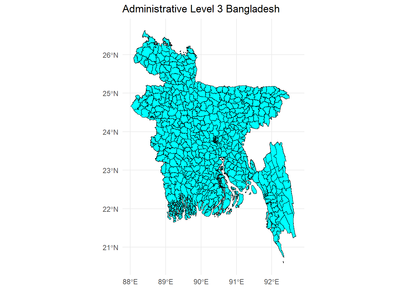

The output gives us the following information about the shape file:

It has 544 features (upazilas) and 16 fields (variables) with information defining the features.
The geometry type is multipolygon. Each multipolygon is a collection of spatial points that define an upazila.
Bounding box shows the extent, i.e. maximum and minimum values of longitude and latitude that define Bangladesh.
As in the case of our base layer, it uses the WGS 1984 datum (EPSG: 4326) geographical projection.
A preview of the first 10 features tells us that for each multipolygon we have information on: administrative codes for the upazila, English name of the upazila, area covered by the shape, and codes as well as names for other administrative levels.

The plot shows a visualisation of the boundaries of each upazila in Bangladesh. They are essentially a collection of multipolygons (i.e. each upazila is bound by a multipolygon object). We will be estimating poverty for each upazila. This illustrates our issue quite nicely - it would be prohibitively costly for a survey like the DHS to travel to each upazila and obtain a sufficient sample size to generate reliable poverty statistics. By using open-source high-resolution remote sensed geo-spatial data, we can model poverty for each zone, including out-of-sample areas, i.e. areas where the DHS did not reach.

We now turn to Steps 2-5, which will process our raster layers of geo-spatial information.

5.4 Steps 2-5 - Write functions for automated processing of geo-spatial covariates

Steps 2-5 all refer to the harmonisation of raster layers that contain geo-spatial covariates. The goal is for all our datasets (accessibility, demographic maps, night lights) to have the same: extent, spatial resolution, and shape as the base layer. In some cases, we may need to additionally address missing values. A detailed description of Steps 2-5 can be found in Section 4.

The reason that all steps are grouped together into one section is that all of those will be performed in a single automated function. We will write two functions, one for accessibility and nightlights data and the second one for demographic maps from Facebook. The only difference between them is the algorithm used for changing the spatial resolution of rasters.

Caution

There are many algorithms that can be used for changing the spatial resolution of a raster, depending on the direction of resampling and types of geo-spatial information represented. We have two cases in our guide:

Accessibility (~250m resolution) and nightlights data (~450 m resolution), which are at a coarser spatial resolution than our base layer (~100m resolution), meaning they have fewer, larger grid cells. Moving from a lower to a higher spatial resolution is called disaggregation, as we see more smaller, or ‘disaggregated’ grid cells in the data after resampling. In this case, we can use the nearest neighbour interpolation method, where each new small pixel is assigned a data value of the older bigger pixel that is closest to it in terms of coordinate location. So, only the data value from one closest grid cell is transferred, and the values from other cells nearby are discarded.
Demographic maps from Meta (~30m resolution), which are at a higher spatial resolution than our base layer (~100m resolution). This means our demographic data has more smaller pixels than the base layer. In this case, we have to “aggregate” a few smaller pixels into a bigger one to match the spatial resolution of our base layer. Given the nature of our data - where each pixel represents the number of people living there - we cannot simply take the value of one closest pixel, as is the case in the neareast neighbour interpolation, because we would discard information on all the other people living in neighbouring cells and underestimate the real population density. Instead, we have to use the “sum” algorithm, which sums up values from all smaller cells that fall within the bigger one (rather than just taking the value from one of them). This way, we will ensure that no people are ‘lost’ when aggregating. In general, the use of the “sum” algorithm is the appropriate method when aggregating (changing to a lower spatial resolution) demographic raster data.

To automate the processing, we will write the first function for processing geo-spatial covariates and call it geo_process. We will use it for the Malaria Atlas accessibility and Nightlights data. It automatically executes the following steps:

Crop your raster to the base layer so that they have the same extent.
Change the spatial resolution of your raster to match that of the base layer using the nearest neighbor interpolation algorithm.
If appropriate, recode missing values to a specified value.
Mask the raster so that it has the same shape as your base layer.

The function requires the following inputs:

aux.raster - this is the raster that you are trying to transform/ harmonise to the base raster layer.
base.raster - your base raster layer that has all the desired attributes. This is the layer we will be harmonising to.
label - the name that you wish to assign to the transformed raster.
value - (if appropriate) the value to which you want to recode NA (missing) values to.

This process will output your transformed raster, ready to be used in the calculation of zonal statistics.

Running the chunk below will create the first function geo_process, which will show up under “Functions” in you environment.

# Function for automating the processing of geo-spatial covariates for use in poverty modelling
geo_process <- function(aux.raster, base.raster, label, value) {

    # 1. Crop to the base layer so they have the same extent
    r <- crop(aux.raster, base.raster)

    # 2. Change resolution to the resolution of the base layer using nearest neighbour interpolation
    r <- resample(r, base.raster, method = "ngb") 
    
    # 3. Replace NA with a specified value (if appropriate)
    r[is.na(r[])] <- value  

    # 4. Select only the shape of Bangladesh as defined by the base layer
    r <- mask(x = r, mask = base.raster)
    
    # Assign a name to the raster
    names(r) <- label
    return(r)
    
}

The second function, called geo_process2 is really similar, but applies the sum algorithm instead of nearest neighbour interpolation when changing the spatial resolution, which is the appropriate method when working with demographic maps from Meta that are of a higher resolution than our base layer. The demographic data from Meta are of a ~30m spatial resolution and require aggregation of the values in each cell when resampled to 100m. Using the nearest neighbour interpolation, we ‘lose’ people (because data is thrown away in the downsample). The’sum’ algorithm instead provides a more accurate representation of population per each 100m grid cell.

Function 2 should be applied to all demographic maps from Meta and will execute the following steps:

Obtain the ratio of spatial resolutions of your layer of interest (from Meta) and the base layer, save those as a factor.ratio.
Crop your raster to the base layer so that they have the same extent.
If appropriate, recode missing values to a specified value.
Change the spatial resolution to match your base layer, on the basis of the ratio defined in Step 1. Note: we are going from a higher to a lower spatial resolution, hence the use of “aggregate”.
Mask the raster so that it has the same shape as your base layer.

Running the chunk below will create the second function geo_process2 and it will show up under “Functions” in you environment.

# Function for automating the processing of geo-spatial covariates for use in poverty modelling
geo_process2 <- function(aux.raster, base.raster, label, value) {
  
    # 1. Get spatial resolutions of both rasters 
    res1 <- res(base.raster)
    res2 <- res(aux.raster)
    
    # Save as a factor of ratios 
    factor.ratio <- res1/res2
    factor.ratio <- factor.ratio[[1]]

    # 2. Crop to the base layer so they have the same extent
    r <- crop(aux.raster, base.raster)
    
    # 3. Replace NA with a specified value (if appropriate)
    r[is.na(r[])] <- value  

    # 4. Change resolution to the resolution of the base layer using the "sum"        algorithm
    r <- aggregate(r, fact=factor.ratio, fun=sum, na.rm=TRUE)

    # 5. Select only the shape of Bangladesh as defined by the base layer
    r <- mask(x = r, mask = base.raster)
    
    # Assign a name to the raster
    names(r) <- label
    return(r)
    
}

Now that we have two automated functions for processing geo-spatial data: geo_process and geo_process2, we can apply it to our raster datasets and create our first visualisations!

5.5 Steps 2-5 - process accessibility data from the Malaria Atlas

In the chunk below, we will process accessibility data from the Malaria Atlas. Those are stored in a list of rasters named matlas.rasters. Simply typing the name of the object tells us more information about each raster in the list, including its class, dimensions, resolution, extent, crs etc. There are three datasets we will be using:

Travel Time to Cities for Bangladesh in 2015
Motorised Travel Time to Healthcae Facilities for Bangladesh in 2020
Walking Only Travel Time to Healthcare Facilities for Bangladesh in 2020.

We will create a new list to store our processed datasets called matlas.processed, then use a loop to apply our geo_process function to all three Malaria Atlas datasets.

# See that all the files have loaded
matlas.rasters

# Now apply this function to a list of rasters from the Malaria Atlas 

# Make a list for storing the processed rasters 
matlas.processed <- list()

# Store the length of the list of rasters
num_r <- 1:length(matlas.rasters)  

# Apply the geo-processing function to all rasters. Here there is no need to replace missing values as 0s (they are already coded as missing), so the parameter for value can stay at NA.
for (i in num_r) { 
matlas.processed[[i]] <- geo_process(aux.raster = matlas.rasters[[i]], base.raster = base.layer.raster, label = matlas.rasters[[i]]@data@names, value = NA)

}

# See the result
matlas.processed

# Compare to base layer
base.layer.raster

Viewing the ready matlas.processed objects, we can see that the dimensions as well as the extent have changed - they are now the same as our base layer.

Now let’s visualise our results! In the code chunk below, I’ll present three ways of visualising geo-spatial layers of information in R:

A simple plot
A high-quality plot image (same as point 1 but manually changing R’s default plot resolution to improve quality)
An interactive html widget using the leaflet package

# Three ways of visualising our data:

## 1. Simple plot ##

# Plot results - with no bounding box or axes, using the viridis colour palette, and adding a main plot title
plot(matlas.processed[[1]], box=F, axes=F, col=viridis(50), main = "Bangladesh - Travel Time to Cities")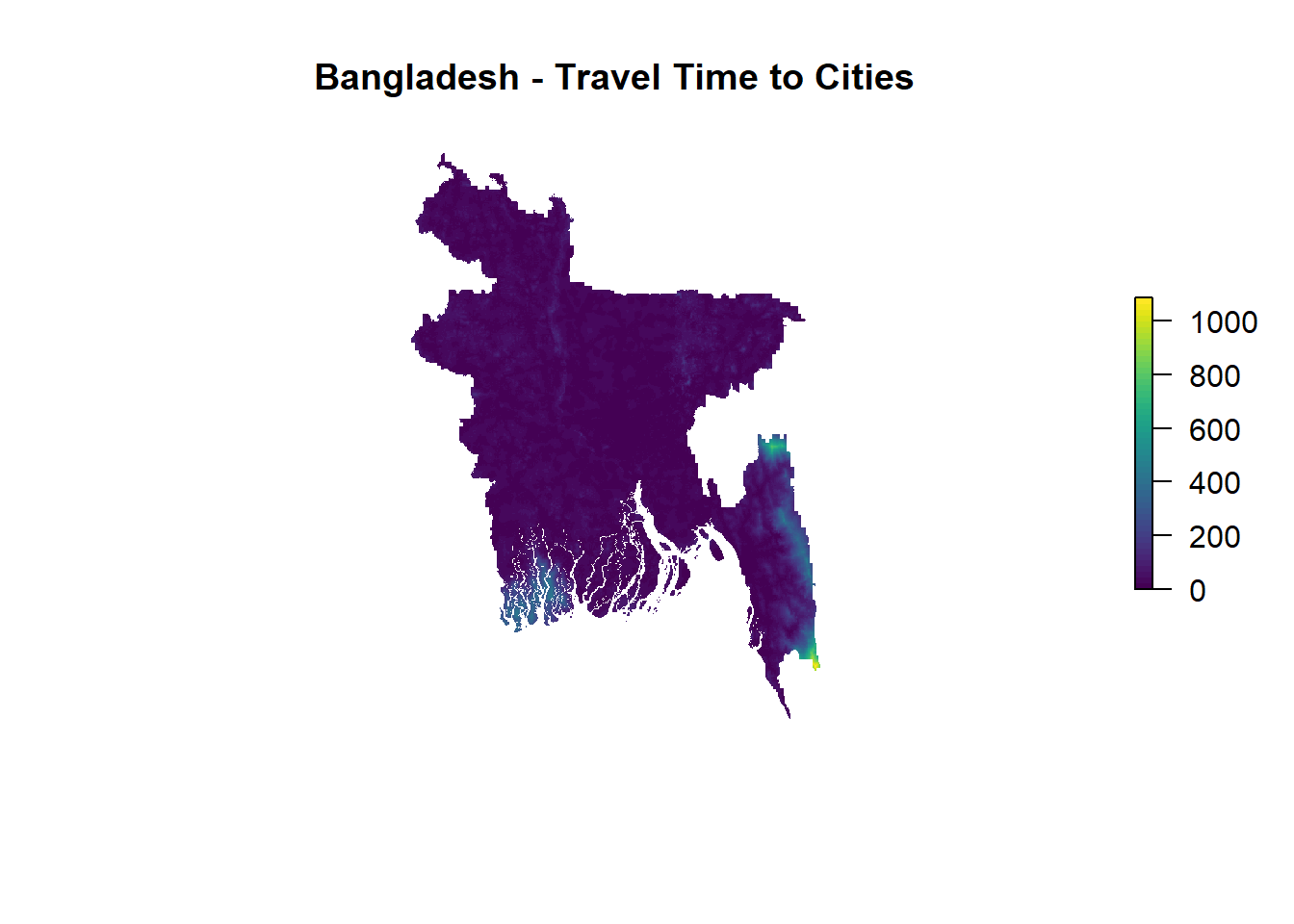

## 2. A high-quality plot image ##

# Create a high quality image - manually changing the resolution of base R plots
png(filename="maps/BGD travel time city.png", res=400, width=2000, height=1500)
plot(matlas.processed[[1]], box=F, axes=F, col=viridis(50), main = "Bangladesh - Travel Time to Cities")
dev.off()

## 3. An interactive html widget ##

# First create a colour palette - let's go with viridis, and supply the values of our raster into domain
pal <- leaflet::colorNumeric(viridis_pal(option = "C")(2), domain = values(matlas.processed[[1]]), na.color = "transparent")

# Create an interactive leaflet map
map_access <- leaflet() %>%
 addProviderTiles(providers$CartoDB.Positron) %>%
  addRasterImage(matlas.processed[[1]],  colors = pal, opacity=0.9, project = FALSE)%>%
  addLegend(pal = pal, values = values(matlas.processed[[1]]), title = "Travel Time to Cities in Minutes")

# Let's have a look
map_access

# Save map as widget
saveWidget(map_access, file="html widgets/BGD_access_map.html")

Let’s start with simple plots. The three plots show visualisations of travel time (in minutes) using the viridis colour palette. Coastal areas as well as western parts of the Chittagong division appear to be least connected to urban areas and healthcare facilities. While this is informative at first glance, a closer zoom in will typically appear quite pixelated. This is because R’s default plot resolution is quite low for high-resolution geo-spatial data. We can change that manually.

In order to view this plot in higher quality, we need to change R’s default plot resolution. The second option will export a higher-quality image of the map showing travel time to cities for Bangladesh and save it in the maps folder in your working directory. Unless you are cloning this repo from GitHub, in which case the folder will already be there, you may need to simply add a folder named maps in your working directory that you specified in Step 1. The high-quality image will be saved there. Now you can zoom into your image and retain much more of the original granularity of the data - but we can step up that visualisation further!

The final approach is creating an interactive map through the leaflet package and exporting it as an html widget. This produces the highest quality visualisation and also allows the end user to interact with our data (for instance, zoom into specific areas of Bangladesh). First, we need to create a colour palette object called pal. Depending on whether we are portraying continuous or categorical data, we will choose the option colorNumeric (for continuous) or colorFactor (for categorical). We then have to supply our colour palette of interest - in this case viridis_pal and define the values that should be assigned to colours, i.e. values of the first raster in the list of processed Malaria Artlas list of rasters matlas.processed[[1]]. Finally, we want NA values to appear transparent.

Once we created the colour pallete, we can start creating our interactive map object called map_access. This relies on Open Street Map base layers that form a sort of “background” on which we will overlay our accessibility data. We select addProviderTiles(providers$CartoDB.Positron), which is a nice light grey shaded OSM global map as the background. There are other options (such as colourful backgrounds) that you can explore. On top of that, we are overlaying the raster image with travel time to cities for Bangladesh. We select the colour palette object pal and opacity=0.9, which controls the transparency of the layer. As the layer already has a specified CRS, we do not reproject. Finally, we add a legend in the viridis colour palette and values of the Malaria Atlas layer. This interactive map is saved in the html widgets folder in the working directory. You can choose any location on your local machine to save this file.

5.6 Steps 2-5 - process the demographic data from Meta

To process the demographic data from Meta, we will apply the second function geo_process2, which relies on the sum algorithm for resampling rather than nearest neighbour interpolation. As before, we will begin by typing the name of the objects that stores a list with all raster files from Meta, fb.rasters. This will allow us to view the properties of the following seven datasets for Bangladesh:

Population Density - Children under 5
Population Density - Elderly 60+
Population Density - General
Population Density - Men
Population Density - Women
Population Density - Women of Reproductive Age 15-49
Population Density - Youth 15-24

Just a note that these datasets use population density per pixel as their unit of measurement. This time, we will be applying our second function geo_process2, which differs only by the type of algorithm that is used for resampling. Since we are working with demographic data of a higher spatial resolution than our base layer, we need to aggregate our data to a coarser grid and the use of the sum algorithm will ensure that we are counting all the populations from all higher resolution pixels. An important step here is replacing missing values with zeros, which is done by specifying the argument value = 0 in the geo_process2 function. From the documentation, we know that pixels which have been coded as missing in fact have no people in it, i.e. the population density is zero - so we can safely recode. However, the user should always check whether recoding missing values as zeros is appropriate.

As before, we create a list fblist.processed, where we will store all the harmonised rasters with demographic information, and apply a loop to process all the seven raster layers with population density for Bangladesh.

# Check that all the files were picked up by this 
fb.rasters

# Make a list for storing the processed rasters 
fblist.processed <- list()

# Store the length of the list of rasters
num_fb <- 1:length(fb.rasters)  

# Apply the geo-processing function to all rasters. Here we need to recode missing values as 0s
for (i in num_fb) { 
fblist.processed[[i]] <- geo_process2(aux.raster = fb.rasters[[i]], base.raster = base.layer.raster, label = fb.rasters[[i]]@data@names, value = 0)

}

# See the result
fblist.processed

# Compare to base layer
base.layer.raster

# Plot results
plot(fblist.processed[[1]], box=F, axes=F, main = "Bangladesh - Population density (children under 5)")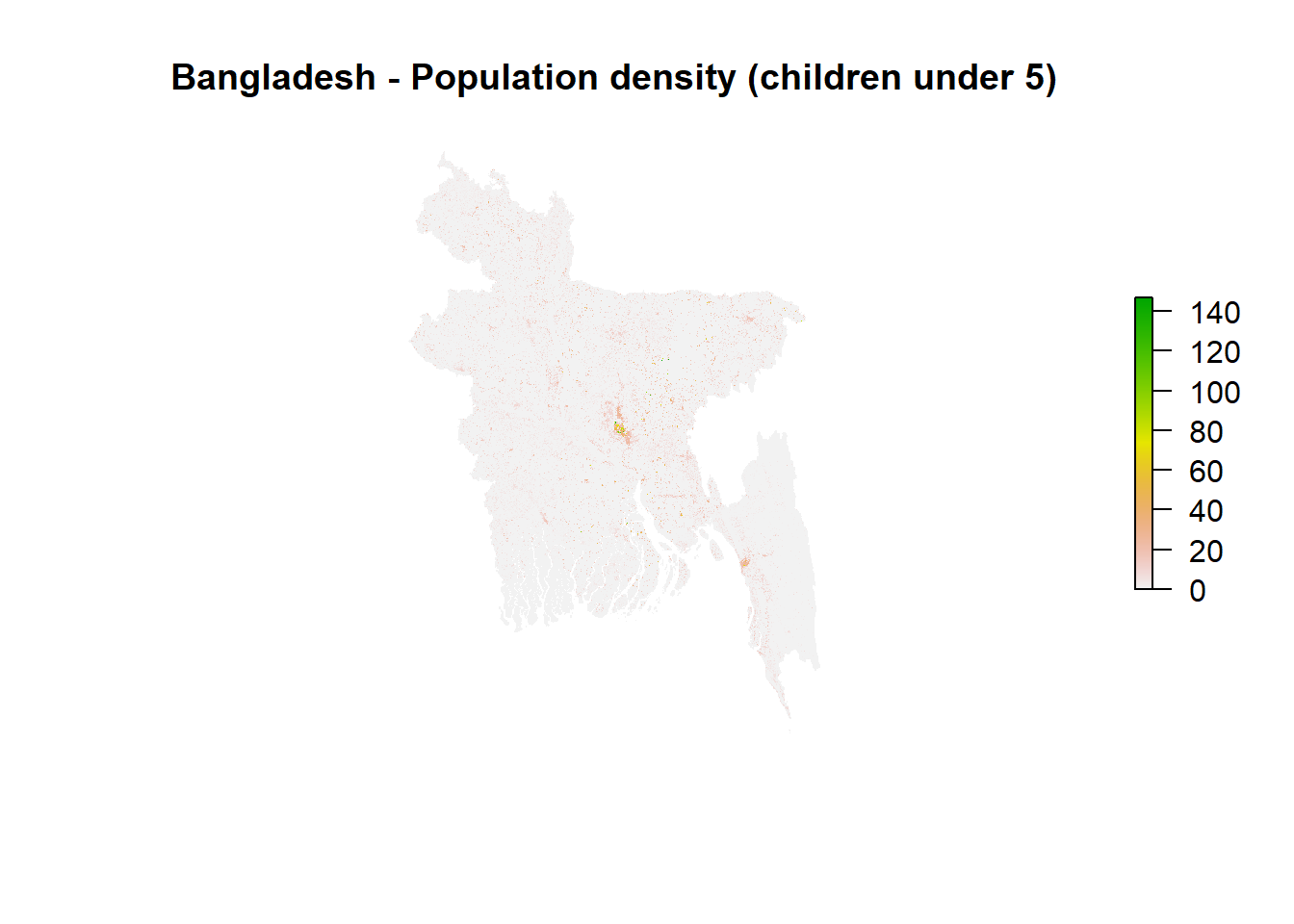

# Create a high quality image 
png(filename="maps/BGD_pop_density_youth.png", res=400, width=2000, height=1500)
plot(fblist.processed[[7]], box=F, axes=F, main = "Bangladesh - Population density (youth 15-24)")
dev.off()

The output from simply typing fb.processed into your console should show you the attributes of harmonised rasters with demographic data from Meta. The dimensions, resolution, extent, CRS should all be the same as the base layer. In addition, we can see the range of minimum and maximum values for each population density raster.

Visualisations show the population density (per pixel) for 7 population groups for Bangladesh. In all cases, we can see that population density increases around urban areas, such as Dhaka or Chattogram. Unfortunately, the size of this raster image is so large that it does not allow us to visualise it using leaflet.

5.7 Steps 2-5 - Process nightlights data

The final dataset that requires harmonisation is the Nightlights Intensity raster from the VIIRS satellite. It contains codified values of radiance per pixel. We will follow the same procedure as with the Malaria Atlas datasets and simply apply our geo_process function. In this case, there is no need to recode missing values. The output, nightlights.raster.processed should again show dimensions, resolution, extent, CRS that are the same as the base layer. In addition, we can see the range of minimum and maximum values of nightlights intensity.

# Apply the geo processing function
nightlights.raster.processed <- geo_process(aux.raster = nightlights.raster, base.raster = base.layer.raster, label = "Nightlights_data", value = 0)

# Check raster
nightlights.raster.processed

# Compare to base layer
base.layer.raster

# Plot raster 
plot(nightlights.raster.processed, axes=F, box=F, main = "Nightlights data in Bangladesh", col=cividis(50))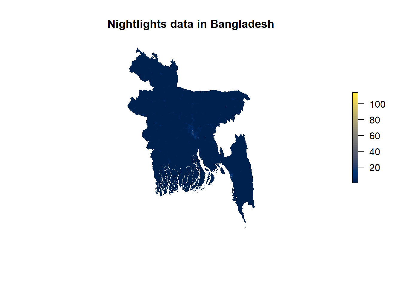

# Create a high quality image 
png(filename="maps/nightlights_BGD.png", res=400, width=2000, height=1500)
plot(nightlights.raster.processed, box=F, axes=F, main = "Nightlights data in Bangladesh", col=cividis(50))
dev.off()

# Create a colour palette

# Set colour palette 
pal2 <- colorNumeric(c("#1A1A1A", "#FD8D3C", "#FED976", "#FFEDA0", "#FFFFCC"), values(nightlights.raster.processed),
  na.color = "transparent")

# Create an interactive leaflet map
map_night <- leaflet() %>%
 addProviderTiles(providers$CartoDB.Positron) %>%
  addRasterImage(nightlights.raster.processed,  colors = pal2, opacity=0.9)%>%
  addLegend(pal = pal2, values = values(nightlights.raster.processed), title = "Nightlights intensity")

# Let's have a look
map_night

# Save map as widget
saveWidget(map_night, file="html widgets/BGD_nightlights.html")

A simple base R plot shows a visualisation of nightlights intensity (measured as radiance per pixel) for Bangladesh using the cividis colour palette. Urban areas such as Dhaka appear to have a higher radiance of nightlights, though it is a little difficult to see given the low default resolution of plots in R. Exporting the plot as a higher-quality image allows for a better visual result.

This could be a good opportunity to introduce custom-made colour palettes into our plots. Instead of using the cividis palette, let’s say we have a very specific idea of how we want to portray the data: black for complete absence of night lights (intuitively, areas that would appear dark in a satellite image), and gradually building shades of yellow that could indicate the presence of lights at night. R Color’s Brewer offers quite versatile palettes for representing all sorts of data: sequential, diverging, and qualitative - and we can construct our own palettes based on these colour schemes. Using the display.brewer.pal command, we can view the colours associated with each palette and using brewer.pal we can obtain their codings. In this case, we want to see the YlOrRd palette and extract the yellow shades, while setting black as the first colour. We save this scheme in the pal2 object and supply it to leaflet. The end result, an interactive html map with my custom colour palette, displays nightlights more clearly.

This concludes our harmonisation of geo-spatial covariates - we now have three lists of rasters that are ready to produce zonal statistics: matlas.processed, fblist.processed, nightlights.raster.processed. As the WorldPop datasets on topography have already been harmonised, there is no need to process them. But we can still play around with some visualisations.

5.8 Steps 2-5 - Inspect pre-harmonised World Pop datasets

The WorldPop datasets already have the same spatial resolution, extent, and dimensions as our base layer. They are ready to produce zonal statistics. Typing the list of raster objects, worldpop.rasters, will show that we have 16 raster objects, with the same attributes as the base layer, all showing distances to different types of Land Cover classes in Bangladesh. We don’t need to further process this geodata in any way - but let’s inspect it by creating simple plots.

As an example, let’s produce a simple base R plot of the 11th raster object from that list, which shows distance to the closest road. Even without any processing, the plot comes out nicely formatted, as World Pop has pre-harmonised this data. Coastal areas are clearly the furthest away from any road. Unfortunately, the raster object is too large to create an interactive map using leaflet.

# See that all the files have loaded
worldpop.rasters

# Check they match the base layer
base.layer.raster

#Plot examples of WorldPop datasets
plot(worldpop.rasters[[11]], box = F, axes = F, main = "Distance to the closest road Bangladesh", col=viridis(50))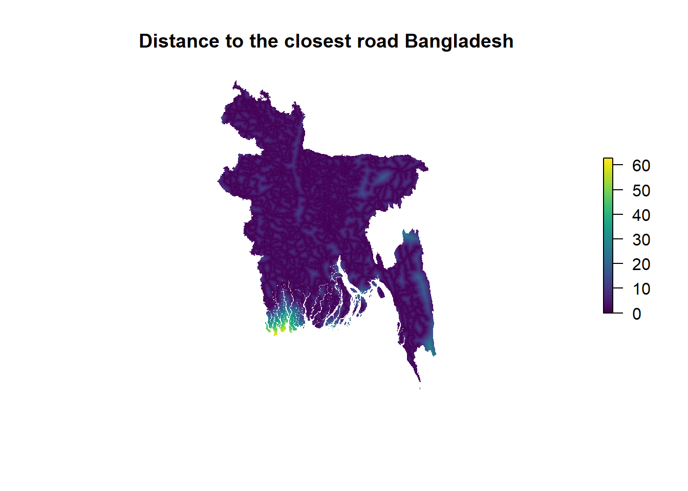

5.9 Step 6 - Calculation of zonal statistics

This brings us to our final step - calculating zonal statistics, i.e. the values of min, max, mean, sd etc. of all the geo-spatial datasets at upazila level, which will serve as inputs into poverty estimation in Section B. For this, we will use our harmonised rasters from steps 2-5: matlas.processed, fblist.processed, nightlights.raster.processed, and worldpop.rasters, as well as the shapefile containing the administrative level 3 (upazila) boundaries in Bangladesh: shapefile.zone.plot.

We begin by putting all of our rasters into one list, full.raster.list and creating a stack of rasters called raster.stack, which is essentially a collection of rasters with the same extent and spatial resolution that can be stored in one file. You can think of those layers as being “stacked” on top of each other. This format will make it easier to calculate zonal statistics as we only have to supply one object to the function (as opposed to doing it separately for 24 raster layers).

Now we can calculate our zonal statistics: mean, minimum value, maximum value, sum, standard deviation, and the number of observations. We will make use of the exact_extract function, which is the quickest and most computationally efficient way of obtaining key statistics from geo-spatial data at the chosen administrative level. Supplying our raster.stack with all geo-spatial data and shapefile.zonal.plot, which contains upazila boundaries in the zonal function will calculate all the statistics of interest. We will save those in a data frame format (which should be fairly familiar!), with column names indicating the zonal statistic for each geo-spatial layer. We will also include a column with the administrative code for each upazila, given by ADM3_PCODE. The name of this final data frame is BGD.zonal.stats.

# Make a list with all the rasters 
full.raster.list <- c(matlas.processed, fblist.processed, worldpop.rasters, nightlights.raster.processed)

# Check rasters 
full.raster.list

# Create a raster stack
raster.stack <- stack(full.raster.list)

# Apply exact extract function
BGD.zonal.stats <- exact_extract(raster.stack, shapefile.zone.plot, c('min', 'max', 'mean', 'sum', 'stdev', 'count'), stack_apply=TRUE, append_cols="ADM3_PCODE")

Congrats! You have made it to the end of Section A on processing geo-spatial covariates. Now you can use them to predict poverty rates for every upazila in Bangladesh, which will be done in Section B.