8 Theory: Key Concepts in Model Fitting
Each step in Section B of the estimation process addresses specific challenges associated with small area estimation using complex survey data. This detailed approach is essential for producing high-quality inputs for area-level models, ultimately leading to better-informed decisions based on the model outputs.
By carefully computing direct estimates and their variances, adjusting for survey design, and applying smoothing techniques, the methodology ensures that the estimates for small areas like upazilas are as reliable and accurate as possible. These steps are necessary because survey data is often produced to be representative at national levels or at administrative division 2 level (district level or urban/rural). In order to generate poverty estimates at more localised levels than this, we need to take account of the sampling strategy used in the household survey and then calculate direct estimates which we can use to complement our model estimates later. These steps are unusual, therefore, in this section, we will explain the theory of the steps so that they make more intuitive sense.
In this guide, we use the 2014 DHS data in Bangladesh for our ground-truth measure of poverty by using the relative wealth index based on asset ownership. Therefore, we will first take a deep look at the DHS sampling strategy.
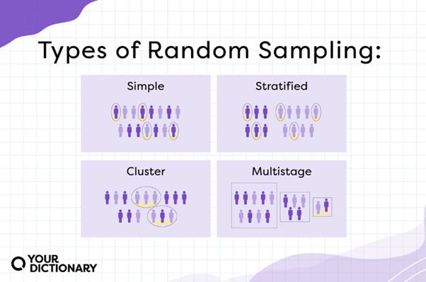
DHS Sampling Strategy
1. Stratification
Stratification involves dividing the population into homogeneous subgroups (strata) before sampling. This ensures that each subgroup is adequately represented in the survey. Stratification can be based on geographic regions, urban/rural status, or other relevant characteristics.
Geographic Stratification: In this case, Bangladesh is divided into districts (not sub-districts/ upazilas which is the small area we want to estimate). Each district is further divided into urban and rural strata.
Urban/Rural Stratification: Separate strata for urban and rural areas within each geographic region.
2. Primary Sampling Units (PSUs)
PSUs are typically geographic areas such as census enumeration areas (EAs) or clusters. These are selected in the first stage of sampling.
- Selection of PSUs: PSUs are selected within each stratum using probability proportional to size (PPS) sampling. The size measure is usually the number of households or the population in the PSU.
3. Household Selection
Within each selected PSU, households are sampled in the second stage of sampling.
Household Listing: A complete listing of households in each selected PSU is conducted.
Random Selection of Households: A fixed number of households (e.g., 30 households per cluster) are randomly selected from the list.
4. Systematic Sampling
Systematic sampling may be employed within the selected PSUs to ensure an even spread of the sample across the PSU.
Why This Sampling Strategy?
Representativeness: Ensures that the survey results are representative of the entire population and various subgroups.
Efficiency: Balances the need for detailed data with practical considerations of time and cost.
Precision: Stratification and multi-stage sampling improve the precision of estimates by reducing sampling errors.

Source: Your Dictionary
However, because the DHS employs these sampling techniques to make the survey representative of the whole population and their specified geographic regions (districts in this case), we need to adjust the estimates in order to use the figures for estimating different areas of interest (sub-districts or “upazilas”). To do this we need to adjust for the sampling design, and calculate direct estimates of the variable of interest, their variance and then smooth this variance.
Direct Estimates
Direct estimates are statistical estimates computed directly from survey data without involving any modelling or external information. For example, if we want to estimate the proportion of households in an upazila that are in the lowest wealth quintile, we can directly calculate this proportion using the survey data collected from that upazila, their respective sampling weights and a stratification adjustment.
Requirement: Direct estimates and their variances are crucial inputs for area-level models, which aim to provide reliable estimates for small areas (upazilas in this case). Accurate direct estimates ensure the overall quality of the model-based estimates.
Objective: To provide reliable initial inputs for further modelling.
Problem Addressed: Without accurate direct estimates, any subsequent modelling would be flawed, leading to unreliable estimates of indicators and their uncertainties.
Variances of Direct Estimates
The variances of direct estimates measure the precision of these estimates. They quantify the sampling variability, indicating how much the estimate would vary if we were to repeat the survey under the same conditions. This is crucial for understanding the reliability of the direct estimates.
Requirement: Surveys often use complex designs involving stratification and multi-stage sampling. Ignoring these complexities can introduce bias in the variance estimation.
Objective: To correctly estimate variances that reflect the survey’s complex design.
Problem Addressed: Mis-estimating variances due to ignoring the survey design can lead to incorrect assessments of estimate precision, impacting the reliability of the area-level models.
Smoothing the Variances
Requirement: Due to small sample sizes, variance estimates can be volatile. Smoothing using Generalised Variance Functions (GVF) helps stabilize these estimates.
Objective: To reduce volatility in variance estimates, enhancing the precision of area-level models.
Problem Addressed: High variance volatility due to small sample sizes can lead to unreliable model estimates. Smoothing provides more stable inputs for modeling.
Process of Smoothing:
Initial Variance Estimation: Compute initial variances, which might be volatile due to small sample sizes.
Regression Model: Fit a generalised variance function to predict variances using predictors such as the number of clusters, sampling weights, and direct estimates.
Application of Model: Use the regression model to smooth the initial variance estimates, especially for upazilas with 2-4 clusters.
Outcome: Stabilized variance estimates, resulting in more reliable model performance.
Why is this important in the Fay-Herriot Model?
Fay-Herriot Model Overview
The Fay-Herriot model is a widely used area-level model for small area estimation. It combines direct estimates from survey data with auxiliary information to produce more precise estimates for small areas. The model is specified as:

where:
Y is the direct estimate for area i.
Theta is the true value of the parameter of interest for area iii
e is the sampling error with variance V(Y)
X is a vector of auxiliary variables for area i.
Beta is a vector of regression coefficients.
u is the area-specific random effect.
- Model Input: The direct estimates (Y) serve as the primary data points that the Fay-Herriot model seeks to improve. These estimates provide the initial, unbiased values for the parameters of interest at the small area level.
- Measurement of Uncertainty: The variances of the direct estimates (V(Y)) represent the uncertainty associated with these estimates. This information is crucial because the Fay-Herriot model uses these variances to appropriately weight the direct estimates and the model predictions. Areas with higher variance (less reliable direct estimates) will rely more on the model-based predictions, while areas with lower variance (more reliable direct estimates) will rely more on the direct estimates.
- Balancing Data and Model: The model balances the direct estimates and the regression predictions based on their respective uncertainties. By incorporating the variances, the Fay-Herriot model effectively combines the information from the survey data and the auxiliary data, improving the overall precision of the estimates for small areas.
- Error Structure: Understanding the variances helps in modelling the error structure correctly. The Fay-Herriot model assumes that the sampling errors are normally distributed with known variances. Accurate variance estimates ensure this assumption is reasonably met, leading to more reliable model outputs.
Summary
Each step in the process addresses specific challenges associated with small area estimation using complex survey data. By carefully computing direct estimates and their variances, adjusting for survey design, and applying smoothing techniques, the methodology ensures that the estimates for small areas like upazilas are as reliable and accurate as possible. This detailed approach is essential for producing high-quality inputs for area-level models, ultimately leading to better-informed decisions based on the model outputs.
Covariate selection to prevent overfitting:

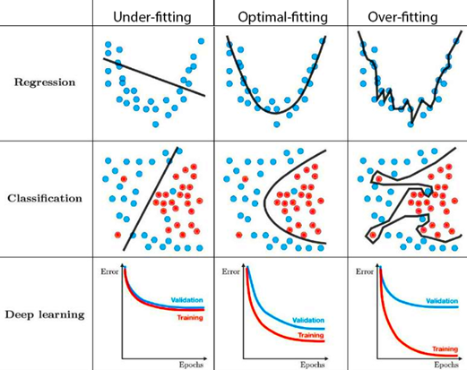
We select only the geospatial covariates with the most predictive power. We do not select all the covariates available because although this would give the lowest error for the small areas with in-sample observations, the model would be overfit and would not perform well in small areas which are out of sample. You can see this example of overfitting by using all the geospatial variables in the right hand column above, in the figure the ‘training’ dataset would represent our in-sample small areas and the ‘validation’ dataset represents the out-of-sample areas since we do not carry out cross-validation in our model fitting process.
If the model is underfit, ie not enough predictive power, the out of sample areas will have a very similar error to the in-sample dataset but neither of them will be good predictions of the actual underlying poverty statistics. This example can be seen in the left hand column and would be the case if we did not use enough geospatial variables to provide predictive power.
We are looking for the optimal-fitting model. For this we use a BIC selection criterion with a penalty with both front and backwise selection. This cycles through adding more and removing geospatial variables until you get the highest predictive power in unseen/ out of sample datasets. In order to do this, we look at the in-sample dataset and build a model iteratively adding and removing different geospatial covariates (with a penalty which ensures you do not use too many covariates) and this generates a model which is the most efficient, provides the lowest error and gives as much predictive power as power. This step is vital since the geospatial covariates are the only resource that the model will have when generating poverty estimates in the next step, therefore, we want to utilise this information as efficiently as possible in the model.
